The Crash at Crush is a perennial go-to narrative in the long-running effort to goad disinterested students into obtaining a much-needed grasp of the the principles of classical mechanics.

From the Wikipedia:

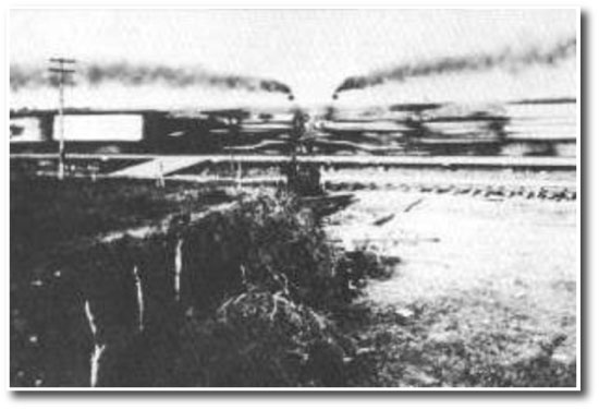
Crush, Texas, was a temporary “city” established as a one-day publicity stunt in 1896. William George Crush, general passenger agent of the Missouri-Kansas-Texas Railroad (popularly known as the Katy), conceived the idea to demonstrate a train wreck as a spectacle. No admission was charged, and train fares to the crash site were at the reduced rate of US$2 from any location in Texas. As a result about 40,000 people showed up on September 15, 1896, making the new town of Crush, Texas, temporarily the second-largest city in the state.

It seems that William George Crush either failed (or more likely never enrolled) in Physics 101. The energy released from the impact of the trains and the explosion of their boilers led to several deaths and many injuries among the 40,000 spectators.

Fast-forwarding 118 years, we find that Stefano “Doc” Meschiari, another Texas entrepreneur, has once again harnessed physics in the name of spectacle with his browser-based video game Super Planet Crash. (Name changed at the last moment from Super Planet Crush in order to duck potential legal challenges from the recently IPO’d purveyors of Candy Crush).

In the time-honored tradition of stoking publicity, a press release was just issued:

April 7, 2014
Contact: Tim Stephens (831) 459-2495; stephens@ucsc.edu

Orbital physics is child’s play with Super Planet Crash

A new game and online educational resources are offshoots of the open-source software package astronomers use to find planets beyond our solar system

For Immediate Release

SANTA CRUZ, CA–Super Planet Crash is a pretty simple game: players build their own planetary system, putting planets into orbit around a star and racking up points until they add a planet that destabilizes the whole system. Beneath the surface, however, this addictive little game is driven by highly sophisticated software code that astronomers use to find planets beyond our solar system (called exoplanets).

The release of Super Planet Crash (available online at www.stefanom.org/spc) follows the release of the latest version of Systemic Console, a scientific software package used to pull planet discoveries out of the reams of data acquired by telescopes such as the Automated Planet Finder (APF) at the University of California’s Lick Observatory. Developed at UC Santa Cruz, the Systemic Console is integrated into the workflow of the APF, and is also widely used by astronomers to analyze data from other telescopes.

Greg Laughlin, professor and chair of astronomy and astrophysics at UC Santa Cruz, developed Systemic Console with his students, primarily Stefano Meschiari (now a postdoctoral fellow at the University of Texas, Austin). Meschiari did the bulk of the work on the new version, Systemic 2, as a graduate student at UC Santa Cruz. He also used the Systemic code as a foundation to create not only Super Planet Crash but also an online web application (Systemic Live) for educational use.

“Systemic Console is open-source software that we’ve made available for other scientists to use. But we also wanted to create a portal for students and teachers so that anyone can use it,” Laughlin said. “For the online version, Stefano tuned the software to make it more accessible, and then he went even further with Super Planet Crash, which makes the ideas behind planetary systems accessible at the most visceral level.”

Meschiari said he’s seen people quickly get hooked on playing the game. “It doesn’t take long for them to understand what’s going on with the orbital dynamics,” he said.

The educational program, Systemic Live, provides simplified tools that students can use to analyze real data. “Students get a taste of what the real process of exoplanet discovery is like, using the same tools scientists use,” Meschiari said.

The previous version of Systemic was already being used in physics and astronomy classes at UCSC, Columbia University, the Massachusetts Institute of Technology (MIT), and elsewhere, and it was the basis for an MIT Educational Studies program for high school teachers. The new online version has earned raves from professors who are using it.

“The online Systemic Console is a real gift to the community,” said Debra Fischer, professor of astronomy at Yale University. “I use this site to train both undergraduate and graduate students–they love the power of this program.”

Planet hunters use several kinds of data to find planets around other stars. Very few exoplanets have been detected by direct imaging because planets don’t produce their own light and are usually hidden in the glare of a bright star. A widely used method for exoplanet discovery, known as the radial velocity method, measures the tiny wobble induced in a star by the gravitational tug of an orbiting planet. Motion of the star is detected as shifts in the stellar spectrum–the different wavelengths of starlight measured by a sensitive spectrometer, such as the APF’s Levy Spectrometer. Scientists can derive a planet’s mass and orbit from radial velocity data.

Another method detects planets that pass in front of their parent star, causing a slight dip in the brightness of the star. Known as the transit method, this approach can determine the size and orbit of the planet.

Both of these methods rely on repeated observations of periodic variations in starlight. When multiple planets orbit the same star, the variations in brightness or radial velocity are very complex. Systemic Console is designed to help scientists explore and analyze this type of data. It can combine data from different telescopes, and even different types of data if both radial velocity and transit data are available for the same star. Systemic includes a large array of tools for deriving the orbital properties of planetary systems, evaluating the stability of planetary orbits, generating animations of planetary systems, and performing a variety of technical analyses.

“Systemic Console aggregates data from the full range of resources being brought to bear on extrasolar planets and provides an interface between these subtle measurements and the planetary systems we’re trying to find and describe,” Meschiari said.

Laughlin said he was struck by the fact that, while the techniques used to find exoplanets are extremely subtle and difficult, the planet discoveries that emerge from these obscure techniques have generated enormous public interest. “These planet discoveries have done a lot to create public awareness of what’s out there in our galaxy, and that’s one reason why we wanted to make this work more accessible,” he said.

Support for the development of the core scientific routines underlying the Systemic Console was provided by an NSF CAREER Award to Laughlin.

I was startled today to learn that a Type Ia supernova has been spotted in M82 — a very nearby, very bright galaxy that even I can find with a backyard telescope. In the image just below, M82 is the galaxy at the lower right.

And here’s a picture of M82 taken yesterday:

Image Source.

The M82 supernova is destined to provide major-league scientific interest. Type Ia supernovae serve as cosmic distance indicators, and yet there are still a number of fundamental unanswered questions about them, including the nature of the precursor white dwarf binary.

Amazingly, it appears that the supernova went unremarked for nearly a week as it increased in brightness by more than a factor of a hundred. Reports indicate that the first team to notice the supernova consisted of Steve Fossey and a group of undergraduate students who were doing a class-related exercise at the University of London Observatory (in the city of London). From the UCL press release (which makes great reading):

Students and staff at UCL’s teaching observatory, the University of London Observatory, have spotted one of the closest supernova to Earth in recent decades. At 19:20 GMT on 21 January, a team of students – Ben Cooke, Tony Brown, Matthew Wilde and Guy Pollack – assisted by Dr Steve Fossey, spotted the exploding star in nearby galaxy Messier 82 (the Cigar Galaxy).

The discovery was a fluke – a 10 minute telescope workshop for undergraduate students that led to a global scramble to acquire confirming images and spectra of a supernova in one of the most unusual and interesting of our near–neighbour galaxies.

Oklo readers will remember that Steve Fossey (along with Ingo Waldmann and David Kipping ) was a co-discoverer of the transits of HD 80606b, work which was also carried out with small telescopes within the London City limits. In February 2009, Steve and I had many e-mails back and forth as he agonized over whether the HD 80606b transit detection had been made with enough confidence to warrant sticking one’s neck out. I always felt a little bad that I advised, what is in retrospect inordinate, caution, having personally experienced several previous bouts of transit fever. As it happened, Fossey, Waldmann and Kipping were barely edged out of making the first announcement by Garcia-Melendo and McCullough and by the French-Swiss team led by Claire Moutou.

So I was thrilled to see that Steve and his students have pulled this one off. I wrote him a quick note of congratulations, to which he replied:

The frantic days of homing in on dear old ‘606 feels like an easy ride, compared to the last 24 hours!

The photometry from the Kepler Mission stopped flowing a while back, but results from the Mission will likely be arriving for decades to come. It’s interesting to look at how the mass-density diagram for planets is filling in. The plot below contains a mixture of published planets scraped from the database at exoplanets.org, as well as a fairly substantial number that haven’t hit the presses yet, but which have been featured in various talks. The temperature scale corresponds to the equilibrium planetary temperature, which is a simple function of the parent star’s radius and temperature, and of the planetary semi-major axis and eccentricity. The solar system planets can be picked out of the diagram by looking for low equilibrium temperatures and non-existent error bars.

It’s especially interesting to see the region between Earth and Uranus getting filled in. Prior to 2009, there were no density measurements for planets in this region, and prior to 2005, there were no known planets in this region. Now there are a couple dozen measurements, and they show a rather alarming range of sizes. A lot of those “terrestrial” planets out there might not be particularly terrestrial.

I’ve written several times, most recently last year, about the Pythagorean Three-Body Problem, which has just marked its first century in the literature (See Burrau, 1913).

Assume that Newtonian Gravity is correct. Place three point bodies of masses 3, 4, and 5 at the vertices of a 3-4-5 right triangle, with each body at rest opposite the side of its respective length. What happens?

The solution trajectory is extraordinary in its intricate nonlinearity, and lends itself to an anthropomorphic narrative of attraction, entanglement and rejection, with bodies four and five exiting to an existential eternity of No Exit, and body three consigned to an endless asymptotic slide toward constant velocity.

This past academic year, I worked with Ted Warburton, Karlton Hester, and Drew Detweiler to stage an interpretive performance of the problem, along with several of its variations. The piece was performed by UCSC undergraduates and was part of the larger Blueprints year-end festival. Here is a video of the entire 17 minute program.

The first of the four segments is an enactment of the standard version of the problem (As set above), and was done with a ballet interpretation to underscore that this is the “classical” solution. Prior to joining the faculty at UCSC, Ted was a principal dancer at the American Ballet Theater, and so the cohoreography was in an idiom where he has a great deal of experience.

The score for the performance was performed live, and is based wholly on percussion parts for each of the three bodies. The interesting portion of the dynamics is mapped to 137.5 measures, which satisfyingly, last for three minutes and forty five seconds.

The nonlinearity of the Pythagorean Problem gives it a sensitive dependence to initial conditions. It is subject to Lorenz’s Butterfly Effect. For the second segment of the performance, we chose a version of the problem in which body three is given a tiny change in its initial position. Over time, the motion of the bodies departs radically from the classical solution, and the resolution has body three leaving with body five, while body four is ejected. A more free-flowing choreography was drawn on to trace this alternate version.

A fascinating aspect of the problem is that while the solution as posed is “elliptic-hyperbolic”, there exist nearby sets of initial conditions in which the motion is perfectly periodic, in the sense that the bodies return precisely to their initial positions, and the sequence repeats forever. In the now-familiar solution to the classical version of the problem, the bodies manage to almost accomplish this return to the 3-4-5 configuration at a moment about half-way through the piece. This can be seen just after measure 65, at which time body 4 (yellow), body 5 (green), and body 3 (blue) are nearly, but are not exactly, at their starting positions, and are all three moving quite slowly:

If the bodies all manage to come to rest, then the motion must reverse and retrace the trajectories like a film run backward. With this realization, one can plot the summed kinetic energy of the bodies, which is a running measure of the amount of total motion. Note the logarithmic y-axis:

The bodies return close to their initial positions at Time = 31, at which time there is a local minimum in the total kinetic energy.

Next, look at the effect of making a small change in the initial position of one of the bodies. To do this, I arbitrarily perturbed the initial x position of body 3 by a distance 0.01 (a less than one percent change), and re-computed the trajectories. The kinetic energy measurements of this modified calculation are plotted as gray. During the first half of interactions the motion is extremely similar, but that the second half is very different. Interestingly, the gray curve reaches a slightly deeper trough at Time = 31. The small change has thus created a solution that is slightly closer to the pure periodic ideal.

I next used a variational approach to adjust the initial positions in order to obtain solutions that have progressively smaller Kinetic energy at time 31. In this way, it’s easy to get arbitrarily close to periodicity. The motion in a case that is quite close to (but not quite exactly at) the periodic solution is shown just below. After measure 65, the bodies arrive very nearly exactly at their initial positions, and, for the measures shown in the plot below, they have started a second, almost identical run through the trajectories.

The perfectly periodic solution occurs when bodies 4 and 5 experience a perfect head-on collision at time ~15 (around measure 33). If this happens, bodies 4 and 5 effectively rebound back along their trajectory of approach, and the motion retraces, therefore repeating endlessly. Here’s the action which shows the collision:

Ted suggested that Tango and Rhumba could be the inspiration for the choreography of the perfectly periodic solution. I was skeptical at first, but it was immediately evident that this was a brilliant idea. The precision of the dancing is exceptional, and the emotion, while exhibiting passion, is somehow also controlled and slightly aloof. No jealousy is telegraphed by motion, allowing the sequence to repeat endlessly in some abstract plane of the minds eye.

We’re putting the finishing touches on a new research paper that deals with an old oklo.org favorite: HD 80606b. The topic is the Spitzer Telescope’s 4.5-micron photometry taken during the interval surrounding the planet’s scorching periastron passage, including the secondary eclipse that occurs several hours prior to the moment of closest approach (see the diagram just below). I’ll write a synopsis of what we’ve found as soon as the paper has been refereed.

In writing the conclusion for the paper, we wanted to try to place our results in perspective — the Warm Mission has been steadily accumulating measurements of secondary eclipses. There are now over 100 eclipse depth measurements for over 30 planets, in bandpasses ranging from the optical to the infrared.

A set of secondary eclipse measurements at different bandpasses amount to a low-resolution dayside emission spectrum of an extrasolar planet. When new measurements of secondary eclipse depths for an exoplanet are reported, a direct comparison is generally made to model spectra from model atmospheres of irradiated planets. Here is an example from a recent paper analyzing Warm Spitzer’s measurements of WASP-5:

Dayside planet/star flux ratio vs. wavelength for three model atmospheres (Burrows et al. 2008) with the band-averaged flux ratios for each model superposed (colored circles). Stellar fluxes were calculated using a 5700 K ATLAS stellar atmosphere model (Kurucz 2005). The observed contrast ratios are overplotted as the black circles, with uncertainties shown. The model parameter kappa is related to the atmosphere’s opacity, while p is related to the heat redistribution between the day and night sides of the planet (Pn = 0.0 indicates no heat redistribution, and Pn = 0.5 indicates complete redistribution).

As is certainly the case in the figure just above, the atmospheric models that are adopted for comparison often have a high degree of sophistication, and are informed by a substantial number of free parameters and physical assumptions. In most studies, some of the atmospheric parameters, such as the presence or absence of a high-altitude inversion-producing absorber, or the global average efficiency of day-to-night side heat redistributions are varied, whereas others, such as the assumption of hydrostatic equilibrium and global energy balance, are assumed to be settled. Invariably, the number of implicit and explicit parameter choices tend to substantially exceed the number of measurements. This makes it very hard to evaluate the degree to which a given, highly detailed, planetary atmospheric model exhibits any actual explanatory power.

The central limit theorem states that any quantity that is formed from a sum of n completely independent random variables will approach a normal (Gaussian) distribution as n becomes large. By extension, any quantity that is the product of a large number of random variables will be distributed approximately log-normally. We’d thus expect that if a large number of independent processes contribute to a measured secondary eclipse depth, then the distribution of eclipse depth measurements should be either normally (or possibly log-normally) distributed. The “independent processes” in question can arise from measurement errors or from systematic observational issues, as well as from the presence of any number of physical phenomena on the planet itself (such as the presence or absence of a temperature inversion layer, or MHD-mediated weather, or a high atmospheric C/O ratio, etc.).

The plot just below consolidates more than 100 existing secondary eclipse measurements onto a single diagram. Kudos to exoplanets.org for tracking the secondary eclipse depths and maintaining a parseable database! The observed systems are ordered according to the specific orbit-averaged flux as expressed by the planetary equilibrium temperaturs — the nominal black-body temperature of a zero-albedo planet that uniformly re-radiates its received orbit-averaged stellar energy from its full four-pi worth of surface area. The secondary eclipse depths in the various bands are transformed to flux ratios, F, relative to what would be emitted from a black-body re-radiator. If all of the measurements were perfect, and if all of the planets were blackbodies, all of the plotted points would lie on the horizontal line F=1.

It’s somewhat startling to see that there is little or no systematic degree of similarity among the measurements. One is hard pressed to see any trends at all. Taken together, the measurements are consistent with a normal distribution of flux ratios relative to a mean value F=1.5, and with standard deviation of 0.65:

This impression is amplified by the diagram just below, which is a quantile-quantile plot comparing the distribution of F values to an N(0,1) distribution.

The nearly gaussian distribution of flux ratios suggests that the central limit theorem may indeed find application, and imparts a bit of uneasiness about comparing highly detailed models to secondary eclipse measurements. I think we might know less about what’s going on on the hot Jupiters than is generally assumed…

One prediction regarding exoplanets that did hold true was the Moore’s-Law like progression toward the detection of planets of ever-lower mass. More than seven years ago, not long after the discovery of Gliese 876 d, the plot of Msin(i) vs. year of discovery looked like this:

With a logarithmic scale for the y-axis, the lower envelope of masses adhered nicely to a straight line progression, pointing toward the discovery of the first Earth-mass exoplanet sometime shortly after 2010. The honors went, rather fittingly, last year, to Alpha Cen B b. Here’s an update to the above plot. Planets discovered via Doppler velocity only are indicated in gray, transiting planets are shown in red…

The data for the plot were parsed out of the very useful exoplanets.csv file published at exoplanets.org.

And wait, what’s going on with that point in 1993? See http://en.wikipedia.org/wiki/Pollux_b.

I think it’s worth making an attempt to coin a term for these “ungiant” planets that are, effectively by default, largely being referred to as super-Earths, a term which brings to mind Voltaire’s remark regarding the Holy Roman Empire.

Planets in the category:

1. Have masses between ~1%  and ~10% of Jupiter’s mass.
2. Have unknown composition, even if their density is known.

Ideally, a term for such planets would:

3. Have a satisfying etymology springing from the ancient Greek.
4. Not be pretentious, or, much more critically, not be seen as being pretentious.

Simultaneously satisfying conditions 3 and 4 is certainly not easy, and indeed, may not be possible. (See, e.g., http://arxiv.org/abs/0910.3989)

I’ve noticed that the esoteric efforts to describe the interiors of these planets — in the absence of any data beyond bulk density — effectively boil down to Robert Fludd’s 1617 macrocosm of the four classical elemental spheres:

This led me to look into Empedocles’ four elements themselves, see, e.g., here. Specifically, can a term of art for the planets of interest be constructed from the original Greek roots?

The following table on p. 23 of Wright, M. R., Empedocles: The Extant Fragments, Yale University Press, 1981, contains various, possibly appropriate, possibilities:

To get going, I had to refer to the rules for romanization of Greek. Initial attempts to coin names (while abundantly satisfying requirement #3 above) have so far failed miserably on requirement #4: chonthalaethian planets, ambroaethic planets, gaiapontic planets. Yikes!

The Tetrasomia, or Doctrine of the Four Elements, alludes to the secure fact that these planets are unknown compounds of metal, rock, ices, and gas. Tetrian planets, maybe? Suggestions welcome…

More than a decade ago, Fred Adams and I wrote a paper that wallowed into the slow motion disasters that can potentially unfold if another star or stars passes through the solar system.

Here’s the abstract:

Planetary systems that encounter passing stars can experience severe orbital disruption, and the efficiency of this process is enhanced when the impinging systems are binary pairs rather than single stars. Using a Monte Carlo approach to perform more than 200,000 N-body integrations, we examine the ramifications of this scattering process for the long-term prospects of our own Solar System. After statistical processing of the results, we estimate an overall probability of order 2×10^5 that Earth will find its orbit seriously disrupted prior to the emergence of a runaway greenhouse effect driven by the Sun’s increasing luminosity. This estimate includes both direct disruption events and scattering processes that seriously alter the orbits of the jovian planets, which force severe changes upon the Earth’s orbit. Our set of scattering experiments gives a number of other results. For example, there is about 1 chance in 2 million that Earth will be captured into orbit around another star before the onset of a runaway greenhouse effect. In addition, the odds of Neptune doubling its eccentricity are only one part in several hundred. We then examine the consequences of Earth being thrown into deep space. The surface biosphere would rapidly shut down under conditions of zero insolation, but the Earth’s radioactive heat is capable of maintaining life deep underground, and perhaps in hydrothermal vent communities, for some time to come. Although unlikely for Earth, this scenario may be common throughout the universe, since many environments where liquid water could exist (e.g., Europa and Callisto) must derive their energy from internal (rather than external) heating.

As one might expect, our scholarly efforts generated only a middling interest from the astronomical community, which soon faded and froze altogether. Science writers, on the other hand sometimes run across the article and write with questions.

I am doing a piece on rogue planets and the scenario that earth might become a rogue planet. I have found some stuff on this on the web and learned that you have done some research on rogue planets.

1. Why do you think rogue planets are so interesting?

From an aesthetic standpoint, there’s something compelling about a world drifting cold and alone through the galaxy, or even through intergalactic space. From a more practical standpoint, if rogue planets are common (as it appears may possibly be the case from the micro-lensing results) it is possible that the nearest extrasolar planet is not orbiting a nearby star, but is rather travelling through the Sun’s immediate galactic neighborhood, say within a few light years of the solar system.

2. Could earth become a rogue planet, and is there any guess, how probable this is? Let’s assume it would happen, what would most probably be the reason for that?

Earth could become a rogue planet if the solar system suffers a close approach by another star (or binary star). If another star passes within ~1 Earth-Sun distance from the Earth, then there is a good chance that the Earth would wind up being ejected into interstellar space. Fortunately, close encounters between stars are extremely rare. There is about a 1/100,000 chance that Earth will suffer this fate during the next five billion years. Those are very low odds, so in the grand scheme of things, we are in an extremely safe position. If we scale the galaxy down by a factor of ~10 trillion, then individual stars are like grains of sand separated by kilometers of empty space, and moving a meter or so per year. It’s clear that in such a system, a sand grain will drift for quite a long time before it comes close to another sand grain.

3. Could you speculate on how a human being on earth would experience the process of earth being kicked out of the solar system?

There would be plenty of warning. With our current capabilities for astronomical observation, the interloping star would be observed tens of thousands of years in advance, and Earth’s dynamical fate would be quite precisely known centuries in advance. The most dramatic sequence of events would unfold over a period of about two or three years. Let’s assume that the incoming star is a red dwarf, which is the most common type of star. Over a period of months the interloping star would gradually become brighter and brighter, until it was bright enough to provide excellent near-daytime illumination with an orange cast whenever it is up the sky by itself. It’s likely that the size of its disk on the sky would become — for a few weeks — larger than the size of the full moon, and vastly brighter. Like the Sun, it would be too bright to look at directly. After several more months, one would start to notice that the seasons were failing to unfold normally. Both the Sun and the Red Dwarf would gradually draw unambiguously smaller and fainter in the sky. After a year, the warmth of the sun on one’s face would be gone, and it would be growing colder by the day… Over a period of several more years, the Sun would gradually appear more and more like a brilliant star rather a life-giving orb. A winter, dark like the Antarctic winter, but without end, and with ever-colder conditions would grip the entire Earth.

4. What do you expect, how long humans could survive such an incident?

The Earth could not support its current population, but with proper planning, a viable population could survive indefinitely using geothermal and nuclear power. We would literally have a thousand years or more to get ready. Certainly, there are much worse things that could happen to humanity.

5. Would any life on earth survive?

Earth would effectively become a large space-ship, and with proper planning, a controlled biosphere (like in a large space colony) could be maintained. Were there no intelligent direction of events, and the Earth was simply left to its own devices, then surface life would freeze away, but the deep biosphere (the oil field bacteria, the deep sea vents, and other other biomes not directly dependent on solar energy) would persist for millions, if not tens of millions of years.

6. What do you think are chances that we will find an earthlike rogue planet?

This depends on what one means by “earthlike”. If one means a planet with Earth’s mass, at very large distance, say thousands of light years, the chances are very good that we will get micro-lensing detections within a decade or so. The data returned, however, will consist only of the likely masses of the planets. Nothing else.

I would estimate that the chances of finding a rogue Earth-mass planet within a potentially reachable distance, say within a light year, are about 10%. The chances, however, that this planet will have an interesting frozen-out surface environment that would please a Hollywood screenwriter are effectively zero. Most rogue planets get ejected from their systems very early in their parent star’s history, long before really interesting things have had a chance to happen from an astrobiological perspective.