The black cloud post describes how the formation of a star and a planetary system can be traced back to the moment when a dense core within a giant molecular cloud begins to suffer an inside-out collapse. The gas at the center of the cloud collapses first, and congregates into the beginnings of a hydrostatically supported protostar. The overlying regions thus lose their support and begin to career inward as well. A wave of collapse radiates outward from the center of the cloud, triggering a downward avalanche of gas and dust. Computer simulations show how gas that has fallen from large distances comes together to form a protostellar disk in orbit around the nascent central protostar. In the image shown below, a simulation of the earliest phases of our own solar system show a region (viewed edge-on) that is several hundred astronomical units across, and plotted 40,000 years after the collapse has started. At this stage of the simulation, roughly half of a solar mass of material has collected in the central protostar, and another half a solar mass or so is orbiting in a very massive protostellar disk.

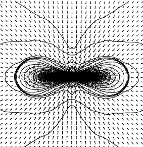
As the disk grows in mass, it begins to feel its own self-gravity, and some regions begin to collapse under their own weight. At the same time, the pressure of the gas in the disk resists the tendancy to collapse, and the differential rotation of the disk acts to sheer out fragments as they grow. This process can also be simulated, and the result is spiral waves (viewed here from above):

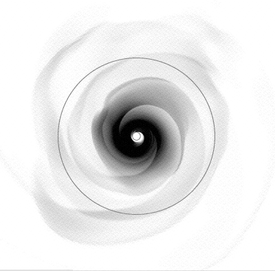
The presence of the spiral waves causes angular momentum to be transferred outward through the disk, while allowing the majority of the mass to flow inward to eventually join with the central protostar. Even after the spiral waves have dissipated, there must exist continuing source(s) of angular momentum transfer through the disk. The identification of these mechanisms is still an active area of research. Possible mechanisms that might operate after the disk is no longer massive enough to support self-gravitating spiral waves include the magneto-rotational instability, as well as convection-driven turbulence in the disk. One way or another, angular momentum transport was extremely effective. The initial cloud that formed our solar system was rotating more or less uniformly, wheras at the present day, there is nearly a complete separation between mass and angular momentum in the solar system. The Sun contains more than 99.8% of the mass, and the planets carry more than 98% of the system angular momentum.

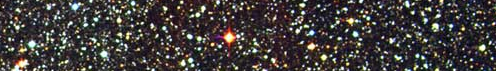
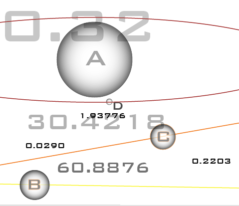
When I give public talks on planet formation, I like to show the above image (taken by HST, and released in 1995) of a protostellar disk, or proplyd, in the Orion star-forming region. We see the cold proplyd from an edge-on vantage, against a diffuse background of hot glowing gas. This disk is at a somewhat later phase of evolution than the ones pictured in the above simulations. It’s roughly 1400 AU across, which is more than 15 times the diameter of Neptune’s orbit, and considerably larger even than the orbits of the newly discovered Kuiper belt objects 2003 UB313, and Sedna. To give an idea of scale, I’ve integrated both Sedna and 2003 UB313 for one Sedna orbit (12,050 years) and plotted their positions relative to the plane of our solar system and superimposed (to scale) on the proplyd. Sedna, is currently in the portion of its orbit where it is speeding (in its rather lazy, loosely bound fashion) through perihelion, and hence the dots plotted at 120.5 year intervals in that region are spaced widely apart. Seen from above, Sedna’s eccentric (e=0.855) orbit would have a aphelion point considerably beyond the radial edge of the proplyd.

Continue reading →