Image Source.

Hey Everybody, if you’ve been working on your fits to the second Systemic challenge system, send them to the e-mail address listed on the web-page given in the Sky and Telescope article.

I’ve been hearing many rumors floating around that there’s going to be a big planet announcement next week. Unfortunately, oklo.org has not yet joined the privileged ranks of the mainstream science press, so I haven’t been privy to any advance looks at the result that’s gonna come off the wire. I did hear, though, that it’s going to be an STScI announcement, so I did a little anticipatory detective work.

STScI runs HST, which means that the result will be the product of Hubble observations. In order to make Hubble observations, one needs to manage to get a block of fiercely competitive Hubble time, which means you need to write a successful Hubble proposal. The abstracts of winning Hubble proposals are posted publicly on NASA ADS. A quick search yields the following accepted proposal abstract (Proposal ID #10466), submitted by Dr. K. C. Sahu:

We propose to observe a Galactic bulge field continuously with ACS/WFC over a 7-day period. We will monitor ~167, 000 F, G, and K dwarfs down to V=23, in order to detect transits by orbiting Jovian planets. If the frequency of “hot Jupiters” is similar to that in the solar neighborhood, we will detect over 100 planets, more than doubling the number of extrasolar planets known. For the brighter stars with transits, we will confirm the planetary nature of the companions through radial- velocity measurements using the 8-m VLT. We will determine the metallicities of most of the planet-bearing stars as well as a control sample, through follow-up VLT spectroscopy. The metallicities of the target stars range over more than 1.5 dex, allowing for a determination of the dependence of planet frequency upon metallicity–a crucial element in understanding planet formation. We will be able to discriminate between the equally numerous disk and bulge stars via proper motions. Hence we will determine, for the first time, the frequencies of planets in two entirely different stellar populations. We will also determine for the first time the distribution of planetary radii for extrasolar planets for both these populations. Parallel observations with NICMOS will provide ultra-deep near-infrared images of a nearby bulge field, which will be used to determine the stellar luminosity and mass functions down to the brown-dwarf regime. The data will also be useful for a variety of spinoff projects, including a census of variable stars and of hot white dwarfs in the bulge, and the metallicity distribution of bulge dwarfs.

I looked at Sahu’s web page at STScI, where he writes:

At present, my research is mainly focused on a large HST program which involves monitoring of about 300,000 stars towards the Galactic bulge using the Advanced Camera System (ACS) on board HST, to search for extra-solar planets. The results are due to appear in the October 5, 2006 issue of Nature.

So clearly, the ACS data have been reduced, and it’s an excellent bet that they’re planning to announce the transit candidates that have emerged from their 7 days worth of ACS photometry. The number of transits to be announced is almost certainly more than two. This week’s announcement of WASP-1b and WASP-2b certainly didn’t produce a noticeable media splash, so there must be a lot of planets in the announcement. And given the past history of HST microlensing planet detections, I bet it’ll be the case that some of the parent stars of the soon-to-be-announced new transiting planets have indeed undergone a fairly rigorous spectroscopic follow-up with the VLT.

I think that spending a whole week of ACS time to stare at stars in the galactic bulge is a fairly worthwhile use of the HST (although I bet a lot of extragalactic astronomers might disagree). Here’s my take: In the mid-1990’s, it was believed that the stars of the galactic bulge are very metal-rich. In 1994, for example, McWillian and Rich 1994 reported an average bulge star metallicity of 0.2 “dex”, that is, ~60% greater than the solar value. More recently, however, Fulbright et al. 2006 have revised the average metallicity of the bulge downward to a value of -0.1 dex (~80% of the solar value). It thus appears that the metallicity distribution of the stars in the bulge is roughly similar to the metallicity distribution of stars in the solar neighborhood.

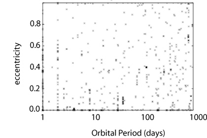
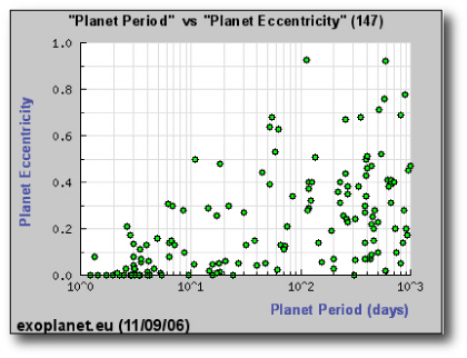
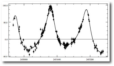
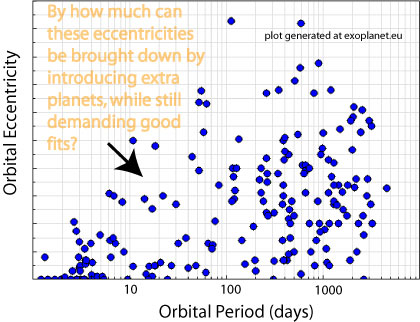
We know from Debra Fischer and Jeff Valenti’s work that the rate of short-period giant planet occurence is a strong function of stellar metallicity:

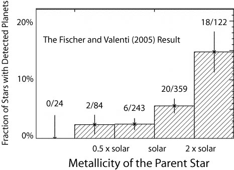
All other things being equal, we can use the above diagram to inform an estimate of the number of planets that Sahu and company will announce. The hot Jupiter occurence rate in a solar-neighborhood type metallicity population is of order 0.7%. About 10% of hot Jupiters will be observable in transit. About half of those transits will be clobbered by the effect of a binary companion sharing the pixel and driving the detection below threshold. For a 7-day survey, about 60% of the hot Jupiters will actually get picked up, given constant coverage and good control of detector systematics (which HST certainly has). This means that Sahu should see (167,000)x(0.007)x(0.1)x(0.5)x(0.6)=35 transiting planets.

The problem, however, will be that there are many events which will look like planet transits, including grazing eclipsing binary stars, transiting M-dwarf stars, and the surprisingly common situation where a background eclipsing binary star shares the pixel with a foreground target star, a so-called blend situation. Dave Charbonneau and his collaborators have written extensively about all of the different pitfalls that can cause a wide-field transit survey to turn up false positives.

So my guess is that there will be of order 200 transit candidates in the ACS data for 167,000 stars. The brightest and most promising of these will have been sent to the VLT for spectroscopic follow-up. If the sensitivity limit of the survey (as stated in the proposal abstract) is V~23, then the candidate stars will likely have V~20-21. Even with the VLT, it’s tough to get accurate radial velocity measurements for stars this dim. So a lack of an observed binary stellar companion will probably be taken as a confirmation of the presence of a planet. (This is all complete speculation on my part.) Going even further out on a limb, my guess is that they have ~100 stars that show transit signatures, and which do not have a spectroscopically detectable binary stellar companion. Although it’ll be hard to further sort the wheat from the chaff, I’ll harbor a guess that 1/3 of the planets that will likely be announced are bona-fide.

Assuming that this is what actually occurs at the press conference, then we’ll have a very interesting result — not so much about the planets (which will be hard to characterize owing to the dim parent stars) — but because of what it tells us about the formation of the galactic bulge. Right now, there are several competing theories for how the bulge formed. One possibility is that scattering of stars by the Milky Way’s galactic bar has populated the Milky Way’s bulge with stars. Another possibility is that the bulge stars are the result of many disrupted globlular cluster or dwarf-galaxy like objects.

A measurement of the planet population of the bulge stars can allow us to distinguish between these two possiblities. If the planet occurance rate is similar to the galactic neighborhood (which I’m guessing will be the gist of the press conference) then the bulge stars are likely to have formed under low-density conditions. This would favor a bar-scattering type of scenario. If the planet occurence rate is zero or very low (which is unlikely, given that they are having a press conference) that would imply that the stars formed in a high-density environment. A crowded star formation leads to a ultraviolet ionizing radiation field that makes it difficult for planets to form and then migrate inward to become hot Jupiters.

There was a remarkable study done with HST in the late 1990s, and published by Gilliland et al. 2000. HST obtained a 8.3-day photometric time series for 34,000 stars in the globular cluster 47 Tucanae. The data, when reduced, show a total absence of transiting planets. This result shows the power of both the environment variable (the 47 Tucanae stars formed in an intensely irradiated region of star formation) and the metallicity variable (the metallicity of the 47 Tucanae stars is about 20% the solar value).

Finally, it’s always good to look at costs. According to the Wikipedia, the total cost of building, launching, servicing, and running HST has been of order 6 billion dollars. It started working as planned in 1994, and will thus have ~15 years of fully functional use. The seven days of ACS time were therefore worth 7.6 million dollars. This is comfortably more than the cost of building a special-purpose telescope to probe the terrestrial planets that are almost certainly orbiting Alpha Centauri B. (For more information, see these oklo.org posts: 1, 2, 3, 4, 5.)

In June 2002, I saw Keith Horne give a review talk at the Scientific Frontiers in Research on Extrasolar Planets Meeting at the Carnegie Institute of Washington. He showed a slide (an updated version of which is here) that listed 23 planetary transit surveys that were in operation at that time. He had asked the investigators running each survey to send him the number of new transiting planets per month that could be expected to turn up. The grand total rang up to a whopping 191 fresh planets per month, or 2,292 planets per year.

For a number of reasons, those numbers haven’t quite panned out, but it nevertheless finally looks like we’re entering a phase where the planetary yield from wide-field transit surveys is starting to ramp up dramatically. Today’s astro-ph mailing has a paper by Collier Cameron et al. entitled “WASP-1b and WASP-2b: Two new transiting exoplanets detected with SuperWASP and SOPHIE”, describing the discovery of P=2.15 d and P=2.52 d planets transiting ~12th magnitude stars. As of this month, astronomers have been hauling in transits at a rate of one per week.

Dave Charbonneau at CfA dropped me an e-mail this morning:

Great chance to catch WASP-1 tonight from the western US. We will pursue it from Mt. Hopkins and Palomar, but thought you might want to give a heads up to transitsearch.org. This one is very much in need of a great light curve, as the current estimates of the planetary radius range from “smallish” to “huge”, with an error bar that is depressingly large.

He’s definitely right about all that. Multiple photometric data sets will be of considerable use in constraining the system parameters. It’s also going to be very important to get a better handle on the properties (Mass, Radius, and metallicity) of the WASP-1b and 2b parent stars. We’d really like to know how these two new planets fit into the overall trends that are starting to emerge among the aggregate of transiting planets.

Ephemerides for both of the WASPs have been added to the transitsearch.org candidates table, and the (rather meagre) published tables of radial velocity measurements have been added to the Systemic back-end. Given the short orbital periods, I don’t think it’ll be very long at all before small telescope observers start producing confirmation light curves.

Image Source.

As we work to get the systemic collaboration off the ground, I’ve been letting transitsearch.org coast along on basically its own devices. That will change fairly soon as we incorporate the transitsearch.org site into the oklo.org backend. This will allow for (among other things) creation of transit ephemeris based on submitted fits, and a tighter collaboration among observers.

In the interim, there’s an important opportunity coming up on October 20th, 2006 for transitsearch.org observers to see whether the highly eccentric planet HD 20782 b can be observed in transit. The a-priori probability is 3.6% that we’ll make a huge (and I mean big deal) discovery. Here’s a link to the oklo post from last April describing the system. I’ll be sending out a campaign notice to the transitsearch.org e-mail list shortly, and I’m hoping that AAVSO will want to collaborate on this campaign as well.

A large number of amateur and small-telescope observers have been catching transits recently. Here’s an overview of some of the results that have showed up in my in-box over the past two months:

Last year, transitsearch.org got an important opportunity to follow up on a high-probability transit candidate. The target was the P=3.34 d planet in the close triple star system HD 188753 that was announced by Konacki, 2005 and which received quite a bit of notice in the press.

Konacki’s planet, which has a minimum mass of 1.14 Jupiter masses, and a predicted radius of ~1.1 Jupiter radii, orbits a 1.06 solar-mass star (HD 188753A) at a distance of ~0.05 AU. The star A is in turn separated by 12 AU (e=0.50) from a binary pair (HD 188753B “a” and HD 188753B “b”). The binary pair B consists of stellar components with 0.7 and 0.9 solar masses in a 155-day e=0.1 orbit (separation of 0.67 AU). The presence of a hot Jupiter orbiting HD 188753A was very surprising, because the presence of the binary B leads to severe difficulties for conventional planet formation theories.

Observations in 2005 by Ron Bissinger and other transitsearch.org observers indicated that it is very unlikely that HD 188753A “b” is transiting (the a-priori probability was 11.8%). Further confirmation of a lack of transits came this July from Joe Garlitz of Elgin Oregon, who writes:

Attached is a chart made from data on HD 188753 taken from 04:45 to 09:30 July 21 [UT]. There is no suggestion of a transit during this time within the capacity of this data. It is difficult to get a good data set since there are no stars within the field at a magnitude similar to HD 188753.

Garlitz’s full figure is here, and his website is here.

One disadvantage of having 200-odd planets rattling around in the planet catalog, is that it’s getting hard to keep all the HD numbers straight. HD 188753 doesn’t show transits, but HD189733 most dramatically does. On July 30th, Donn Starkey, of Auburn, Indiana sent a nice light curve of HD 189733 during the JD 2453946.7 transit:

More detail regarding Starkey’s results can be found on his website.

On August 27th, I received a dispatch from Veli-Pekka Hentunen of Varkaus Finland. Summer has finally wrapped up in Finland, and Taurus Hill observatory (featured in this post from last May) is again open for business:

Last weekend, we began to continue exoplanet transit observing after the long Finnish light summer. On the night of August 26-27 w observed our first XO-1b transit at the Taurus Hill Observatory, Varkaus (obs. code A95). We were able to catch only about half of the entire transit because the object was quite low in the north-western sky, and the altitude decreased from 30 to 15 degrees during the course of observation. Our light curves and observing information are given on our English website.

In a follow-up e-mail on September 17th, Hentunen reported that they had observed a full transit for HD 189733 on the night of September 16th-17th:

Starting on September 9th, Tonny Vanmunster, Kent Richardson, and Ron Bissinger all reported observations of the newly discovered TrES-2 transit. Tonny and Kent’s observatons are detailed in this oklo post, whereas Ron’s TrES-2 light curve looks like this:

Don Carona at Texas A&M also sent a light curve of a TrES-2 transit, obtained (under less-than-ideal weather conditions) from the Physics Dept. at College Station. Here’s an unbinned excerpt from his reduced high-cadence time series:

Notice the the lack of a flat bottom for the TrES-2 transit (which is more obvious to the eye when the data is binned). TrES-2 crosses the star with a high “impact parameter”, which means that the planet does not occult the central portion of the star as seen from Earth. Stellar Limb Darkening is responsible for the remarkable smoothness of the dip.

On September 19th, Bob Buchheim of Altimira Observatory sent a very nice HD 189733 lightcurve:

Along with the photometry, he sent a report of an entirely new strain of transit fever:

Last night I monitored HD189733 for a photometric transit signature. A bit of an embarassing story: I noticed that it was nicely placed and “in window”, so I set up the telescope and went to bed … but I forgot to check if transits had already been detected for this star. Imagine my surprise at the resulting deep transit signature! (See attached graph). Oh, well, now that I’ve checked, I see that I’m a year late with this “discovery”.

Bob’s experience reminds me that I’ve got to update the various results pages for the transiting candidates. The transitsearch results page for HD 189733 b reports (erroneously, and by default) that “No photometric transitsearch has yet been reported for this system”. Yikes!

Finally, just a few minutes ago, I got an e-mail from Arto Oksanen, who was the first amateur to observe an HD 209458b transit (on Sept. 16th, 2000). Six years later, it looks like he’s also the first amateur to observe HAT-P-1b

I observed the end of transit of HAT-1b last night at Hankasalmi Observatory, Finland. The weather was not very good, but the egress was well visible. The observing instrument was a 40 cm RC telescope. I used V-filter with SBIG STL-1001E CCD.

Oksanen’s light curve is plotted is at this link, and is reproduced just below:

Oksanen notes that the egress seems to occur 30 minutes early relative to the published ephemeris. This could well be the case. The longer the time baseline for transit observations, the more accurate the ephemeris become. Small-telescope observations have an important role to play in this regard.

Image Source.

Chalk another transiting exo-planet up on the board. In a preprint released today, Gaspar Bakos and his colleagues in the HATnet project are announcing HAT-P-1b, a large-radius, low-density planet transiting one member of a relatively nearby, relatively bright solar-type binary star.

HAT-P-1b (which orbits the star BD+37 4734) is quite interesting for several reasons. Its 4.46529 day orbit is the longest period yet detected for a transiting extrasolar planet, and its measured radius of 1.36 Jupiter radii is alarmingly larger than the baseline theoretical prediction. The planet contains 0.53 Jupiter Masses, and has a surface temperature near 1100 K, so our models predict that it should have a radius of 0.94 Jupiter radii if it contains a 20 Earth-mass heavy-element core, and a radius of 1.09 Jupiter radii if it’s made of pure solar-composition gas. It’s thus roughly 20-30% larger than it “should” be, which means that something is providing it with a very significant source of extra interior heat.

The large radius of the planet means that the transits exhibit a ~1.5% photometric depth. Deep transits make it easier to obtain data with high signal-to-noise, which means that we can look forward to very accurate follow-up measurements for this system. The presence of a nearly identical companion star at a separation of 11 arc seconds should also help observers obtain good differential photometry. The star is up now, and its well-placed for Northern Hemisphere observers. I don’t think it’ll be long before we see confirmations rolling in from small-telescope observers worldwide. If you’re interested in observing it, the ephemeris table is here.

Where could the extra source of heat be coming from? One possibility is tidal dissipation related to the circularization of an eccentric orbit.

The theory of tides can rapidly slip into thousands of pages of detailed mathematical analysis. Many of the interesting ideas, however, are close to the surface. In the introduction to his still-useful 1898 popular book, “The Tides”, Sir George H. Darwin, the son of the naturalist, and Plumian Professor at Cambridge, wrote:

A mathematical argument is, after all, only organized common sense, and it is well that men of science should from time to time explain to a larger public the reasoning behind their mathematical notation. To a man unversed in popular exposition it needs a great effort to shell away the apparatus of investigation and the technical mode of speech from the thing behind it.

I would actually argue that the situation is quite the opposite. I think it’s easier and better to get a colloquial, heuristic understanding first, and then make an attempt to put the ideas on a sound mathematical basis.

For a planet that (like Hat-P-1b) has an orbital period of less than a month or so, it’s expected that tidal forces will rapidly bring the planet into synchronous rotation, in which the planet spins once on its axis every orbital period. For a circular orbit, this means that the planet always keeps one face to the star, just as the Moon keeps one side toward the Earth. If the orbit is eccentric, however, the planet will not manage to keep one side directly facing the star. Because the planet spends more time at the far point of its orbit, it does more “turning” there, and remarkably, it turns out that the planet always keeps one face pointed toward the empty focus of its elliptical orbit. From the point of view of the star, a fixed point on the planet is seen to librate. The Moon’s orbit is slightly eccentric, and so we can see this effect in time-lapse animations of lunation. See here and also (if you’re not inclined to motion sickness, here).

The tidal bulge of the planet, on the other hand, is forced to always point toward the star, as it’s the star’s gravity that is producing the differential gravitational attraction. This means that once per orbit, the tidal bulge is rocked back and forth across the planet, which produces serious internal heating. The size of the bulge also increases and decreases once per orbit due to the varying distance between the planet and the star, and the resulting oscillation also contributes to the amount of internal tidal heating.

The amount of tidal energy deposited in the planet increases with the square of the orbital eccentricity. A reasonable model for the physical properties of HAT-P-1b indicates that an eccentricity e=0.09 is adequate to generate enough tidal heating to expand the planet to its observed size of 1.36 Jupiter radii. The problem, is that the orbit should circularize on a timescale of less than 1 billion years, whereas the system seems to be about 4 billion years old. Therefore, if a significant orbital eccentricity exists, then there must be a mechanism to maintain the eccentricity. The best candidate is another planet further out in the system.

We can take a quick look to see whether such a situation holds water. A second planet in the system will exert gravitational perturbations of HAT-P-1b, which will cause its eccentricity to vary with time. The picture to have in one’s head is to imagine that the planets are viewed on a timescale that is much longer than an orbital period. If one takes the long view, the motion of the planet is effectively blurred out along the orbit, and one can model the planet as an elliptical wire of varying mass density — heavy near apastron where more time is spent, and light near periastron where the planet spends less time. The interaction between the two planets can then be modeled as the interaction between two flexible elliptical wires. When one does this, and ignores the moment-by-moment motion of the planet, one is making a “secular approximation”. Secular theory was developed to a high art in the 1770s by Laplace and Lagrange, and we can make use of their work to quickly look at how the eccentricities of two mutually interacting planets vary with time.

Over at the transitsearch.org, I have a program which computes a 2nd-order secular theory for each of the known multiple-planet systems, and plots the resulting eccentricity variations as part of the candidate information table . (To see the plots of the secular variations, click on the “planet column” for a multiple planet system such as Upsilon Andromedae).

An advantage of using the secular approximation to the dynamics is that one can quickly scan through a range of planet-planet configurations and find out what the perturbative interactions look like. If I add a second planet to the HAT-P-1 system with a period of 50 days, a mass of 0.06 Jupiter masses, and an orbital eccentricity of e=0.30, I get the following long-term variation in eccentricities, in which the eccentricity of planet b has a time-averaged value close to e=0.09:

Is it possible to hide a second planet in the system while remaining consistent with the (still sparse) set of published radial velocity measurements? The downloadable console is ideally suited to quickly answering such a question. It turns out that it’s very easy to get a perfectly adequate 2-planet fit to the data in which a hypothesized perturbing outer planet is capable of maintaining a time-averaged eccentricity e=0.09 for the inner planet. One such fit looks like this:

corresponding to a system configuration that looks like this:

It would be exciting if a planet like the one in the above diagram (or its dynamical equivalent) could be detected. This would tell us that we’re on the right track in obtaining a better understanding of the wide range of observed radii among the known transiting planets. Probably the fastest way to detect the perturbing planet is through accurate timing of the intervals between successive transits. If an outer planet is tugging on the inner planet, then the orbit will fail to be perfectly periodic, and variations will be observed in the amount of time that passes between transits. Matt Holman and Norm Murray have written a paper that describes how this works. They give a rule-of-thumb equation for the transit-to-transit variations that one can expect. For a planet similar to HAT-P-1b, with semimaor axis a1 and period P1, and a pertubing planet with simimajor axis a2 (where a2>a1), period P2 and mass M2, they find that the typical variation of the interval between successive transits is given by

where

For HAT-P-1b and HAT-P-1c (as hypothesized above) delta T works out to about 5 seconds. Variations of this magnitude are readily detected from the ground, and a number of research groups will probably jump right on this problem.

The transit game is getting to be a competitive global business. No sooner is a new transit announced than amateur astronomers worldwide are on the sky to obtain follow-up observations. Tonny Vanmunster, of Landen Belgium and Ron Bissinger of Pleasanton California are generally among the first to check in with confirmations. Vanmunster nailed TrES-1 a mere week after its announcement in 2004. Last summer, Bissinger caught HD 149026b on literally the day it was announced. In the case of TrES-2, which was announced yesterday, it looks like Vanmunster has snagged the prize. “What’s up, Cali?”

[Actually, it was both cloudy and the middle of the day in Pleasanton while Vanmunster was on the sky. But there’s a transit tomorrow night, Sept. 10/11 PDT, that Ron’ll likely catch.]

Here’s Vanmunster’s light curve. The transit was in progress at dusk in Belgium, so he was able to observe only the latter part of the event.

Vanmunster writes:

Here are some technical details : observations were made at CBA Belgium Observatory, using two 0.35-m f/6.3 Celestron telescopes, each equipped with an SBIG ST-7XME CCD camera. I simultaneously made unfiltered and R-band observations (hence the 2 telescopes). The included light curve is unfiltered, and each dot in the curve is the average value of 5 successive observations (binned). The gray lines show the standard deviation (about 4 millimag on average). Exposure time was 15 to 20 sec.

The egress is very evident in the light curve, and happened right at the predicted time. The transit depth was approx. 0.0155 mag, which again corresponds well with the value published in the discovery paper.

Follow-up observations such as the ones made by Vanmunster and Bissinger can be very scientifically useful. For example, Vanmunster’s 2004 observations allowed us to get an improved estimate of the TrES-1 planetary radius, and he co-authored a journal article with us on that topic. Both Vanmunster and Bissinger were involved in the discovery of X0-1, and both are co-authors on the recent Shankland et al. paper which I’ll talk up in an upcoming post.