Douglas Adams single-handedly elevated the number 42 to a prominence that it otherwise certainly wouldn’t have.

Not that the atomic number of molybdenum should lack importance. Forty two, moreover (and change) is the number of minutes required to fall through a uniform density Earth in the event that a frictionless shaft were to be somehow dug through the globe.

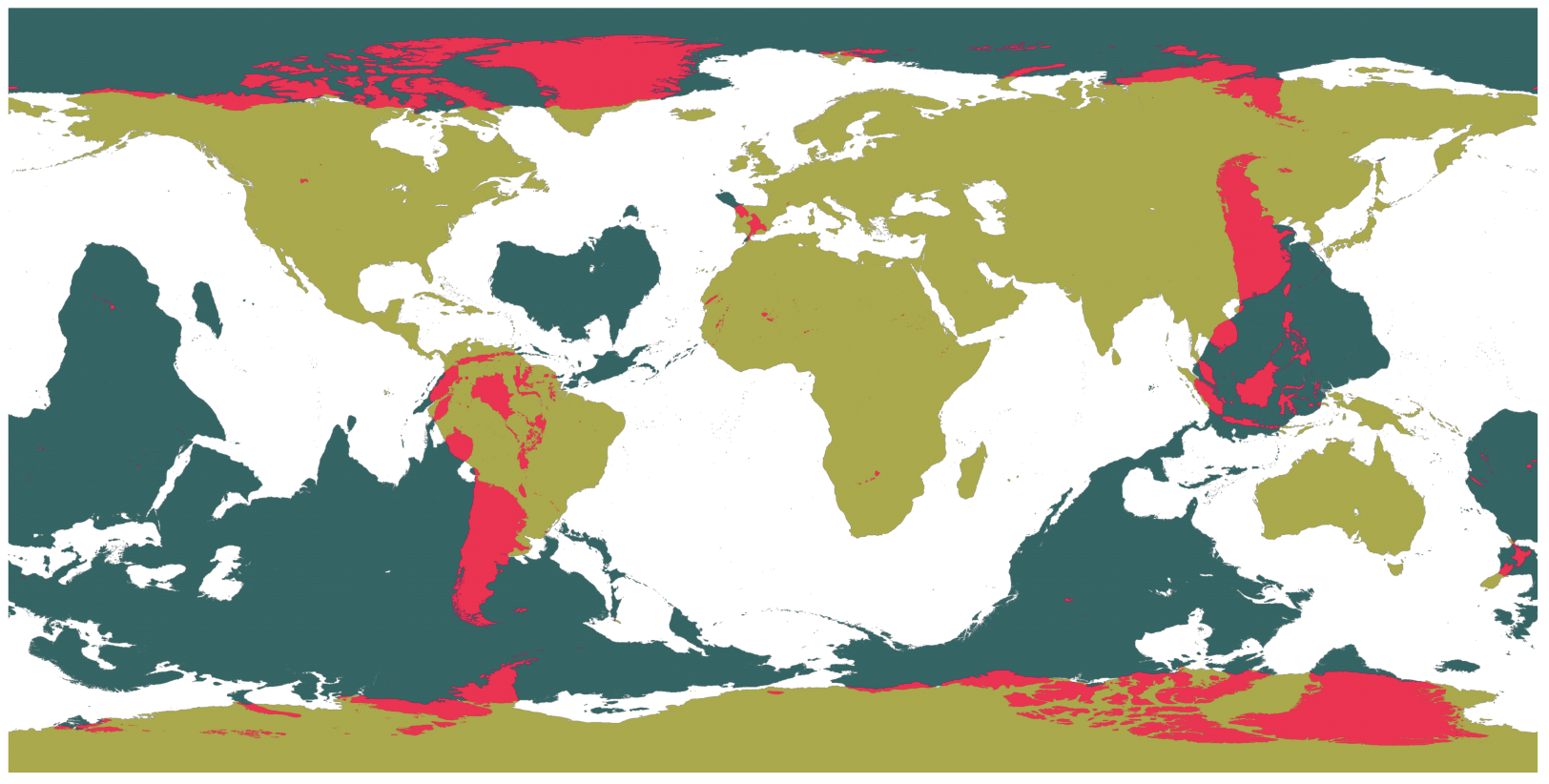
The issue of falling through the Earth naturally proceeds to the antipodal map. That is, where do you come out if you tunnel vertically?

If you’re reading this in North America, you come out in the Indian Ocean, hundreds to thousands of miles from Perth Australia, the nearest big city. The one exception is locations just north of the Sweet Grass Hills of Montana:

which are antipodal to Kerguelen:

In fact, if you’re reading this on land anywhere on Earth, your odds of not emerging in the ocean are rather slim. Only three percent of the globe is comprised of land that is antipodal to land. In essence, the cone of South America runs through China into Siberia on the antipodal map.

Staring at the map reveals some curious asymmetries. Look at how Australia nestles into the Atlantic, and how Africa fits into the Pacific. Is this just a random superposition? On average we’d expect three times as much land to be antipodal to land than is the case with the present-day Earth. Is this a “thing”, or is it simply a coincidence?

The andecdotal land-opposite-ocean observation can be analyzed by decomposing the Earth’s topography into spherical harmonics and analyzing the resulting power spectrum. In 2014, I wrote an oklo.org article that looked at this in detail. Mathematically, the antipodal anticorrelation — the tendency of topographical high points to lie opposite from topographical low points — is equivalent to the statement that the topographical power spectrum is dominated by odd-l spherical harmonics.

Arthur Adams and I have been looking into the antipodal anti-correlation off and on for a number of years, and have worked up some theories that are almost certainly incorrect (as are essentially all theories that involve and then in their initial construction). Nonetheless, they are provocative and polarizing, and so thus appropriate to the jaded sensibilities of oklo.org’s sparse readership of scientific connoisseurs.

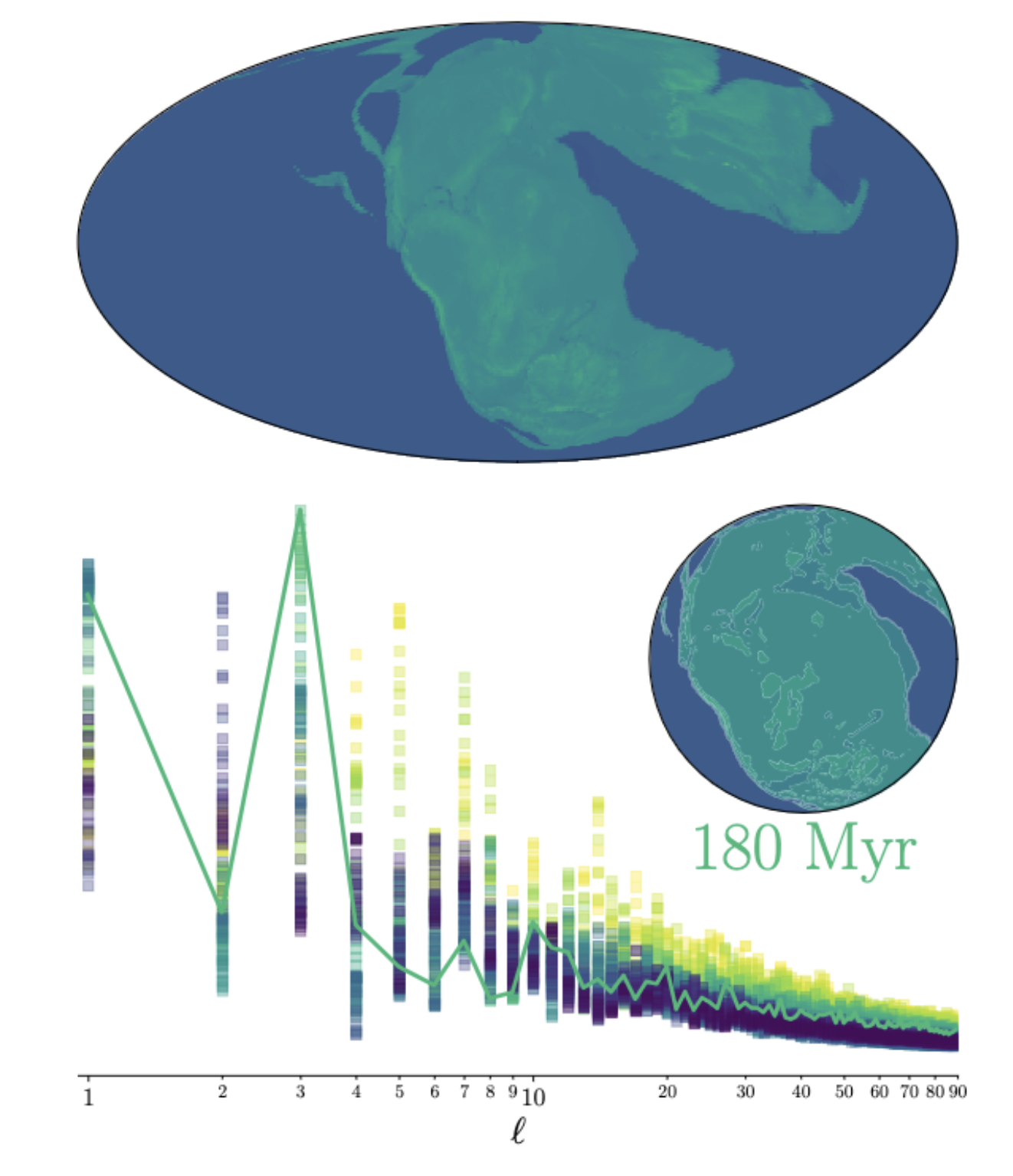
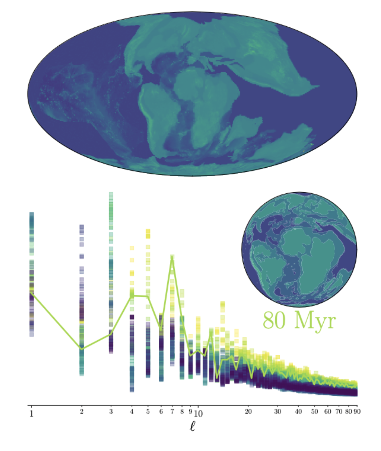
To start, the antipodal anti-correlation has been around at least since the Carboniferous. Paleo digital elevation models exist, and so we can look at the evolution of the topographical power spectrum through time:

Since roughly 330 million years ago, when the super-continent Pangaea first assembled, the elevation spectrum has exhibited strong powers in the l = 1 harmonic (peaking about 320 million years ago), at the l = 3 harmonic (peaking about 180 million years ago), at the l = 7 harmonic (peaking about 80 million years ago), and most recently at the l = 5 harmonic, which peaked about 10 million years ago and which continues to the present day. The current net anti-correlation is actually near its minimum strength relative to the last few hundred million years of Earth’s history. Is there a physical reason for this marked preference for odd-l modes?

Image Source

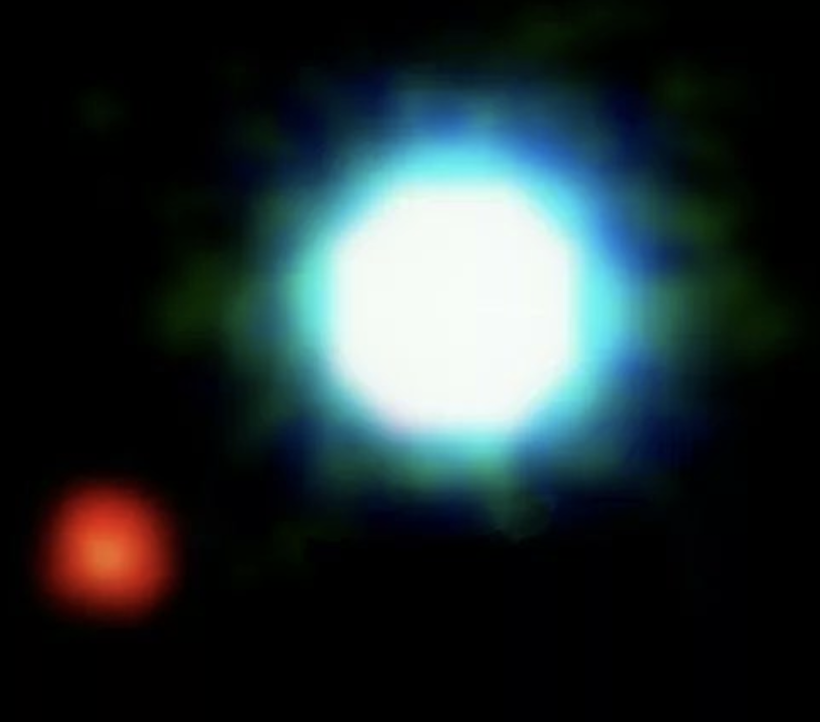
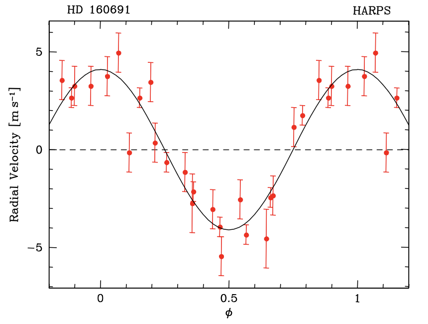
Two decades ago, a brisk list of a hundred-odd alien worlds comprised the entirety of the extrasolar planet census. HD 209458b, along with a faintly dubious handful of OGLE objects, were the only exoplanets known to transit, and the Doppler radial velocity technique was unambiguously the go-to detection platform. The picture just above (discussed further below) had also just been released. The California-Carnegie Team, with their running start and their Keck access, seemed to occupy the driver’s seat. In the course of a ten-year run, they bagged dozens upon dozens of planets. There is a time-capsule feel to the team’s forgotten yet still-functioning website, which includes a planet table frozen to the start of 2006.

Competition in the Doppler arena was nonetheless keen. The HARPS spectrograph had begun collecting on-sky measurements in 2003, and by August of 2004 it was exhibiting the meter-per-second long-term precision needed to reliably announce the first super-Earths. This graph from the Geneva Team was (and still is) genuinely stunning.

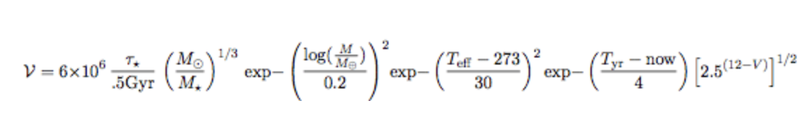
Gradually, however, transit photometry began displace the radial velocity technique. Transit surveys benefit from the massive parallel processing of stars, and fewer photons are required to secure strong candidate leads. In theory, at least, transit timing variations obviate the need to obtain velocities. Transiting planets are vastly more amenable to characterization. I tried to quantitatively capture this shift with a valuation formula for planets that was normalized in expectation to the 600-million dollar cost of the Kepler Mission:

I excitedly strung together a series of articles starting with this post that discuss the various terms of the formula. It places a stringent premium on demonstrably Earth-like qualities, and its exponential terms are unkind to pretenders within that slippery realm of habitability. Mars, in particular, prices out at $13,988.

Over time, I lost interest in trying to promote the formula, and indeed, I began self-reflecting on “outreach” in general. There was a flurry of less-than-attractive interest in 2011, including a sobering brush with the News of the World tabloid shortly before its implosion in July of that year.

GPT-4’s facility with parsing online tables makes short work of assessing how the present-day census of more than five thousand planets propagates through to a list of valuations. The exercise is interesting enough that I’ll hold it in reserve. At quick glance, it looks like Proxima-b was the first planet to exceed the million-dollar threshold, despite the expectation that the Kepler Mission would detect worlds worth thirty times as much.

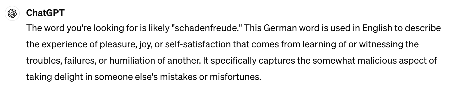
Somewhat ironically, the exoplanets managed last year to trigger some serious destruction of economic value. As we know, the language models are prone to making stuff up. So it’s important to get out there and check their work. Google had the misfortune of being side-swiped by astro-twitter, which crowed with ______ (see just below) when Bard’s trillion-odd weights and biases somehow failed to grasp that the ~5 Jupiter-mass companion orbiting the ~25 Jupiter-mass brown dwarf 2MASSWJ 1207334-393254 is technically an extrasolar planet.

From the Reuter’s article describing the disaster:

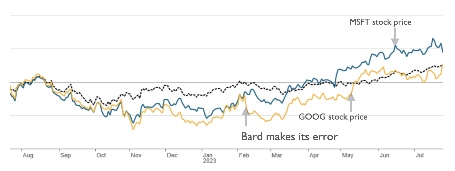
“Google’s new Bard system appeared to fall victim to that pitfall on Monday when an example the company posted of its responses claimed that the James Webb Space Telescope took “the very first pictures” of an exoplanet outside the solar system. The National Aeronautics and Space Administration says on its website that the first images of an exoplanet were taken as early as 2004 by a different telescope.”

As a direct result of the blunder, Google’s stock fell 7.7%, which destroyed 99.8 billion dollars in market capitalization, more than the combined market value of Ford and GM, and about ten times the all-in cost of JWST itself. Comparison of the subsequent evolution of Google’s and Microsoft’s stock prices suggest that the exoplanet-induced loss was effectively realized, and was not just a mean-reverting shock.