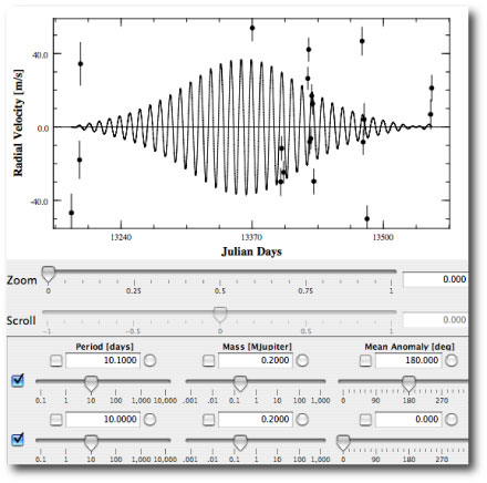
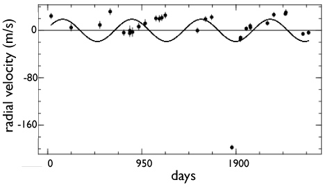
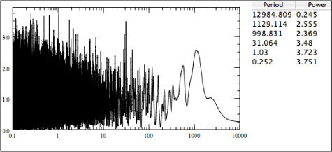
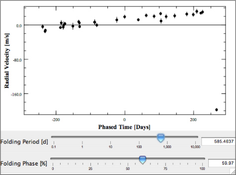
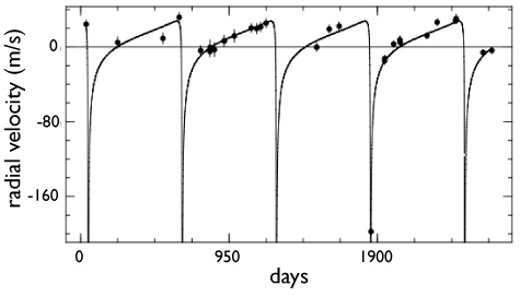
Ups and Downs and Ups And

Visitors to oklo.org may have noticed that the site was down for most of Sunday. I’d been neglecting to update my WordPress installation, which lead to a problem with the database, and a huge load spike for the server. Everything seems stable now, and I’m now flossin’ 2.8.4 inch rims.

In the relatively near future, I will be modernizing some aspects of the look and feel of the site, which will make it more discussion-friendly, and more smoothly slotted into the hum of the outside world. No need to worry, though. We’ll continue to roll ad-free.

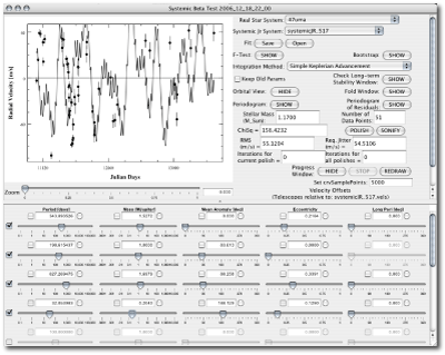
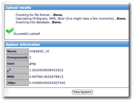
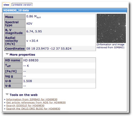
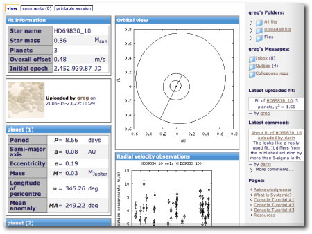
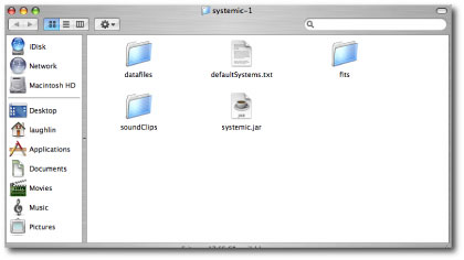
I’ve updated the second systemic console tutorial which guides the user through the remarkable Upsilon Andromedae radial velocity data set. The back-end database is getting closer to its relaunch, and the systemic console (version 1.0.97) is freely available for download here.

Read on to work through the tutorial.

Continue reading

the pause that refreshes

The systemic backend will be offline for a period of time starting on Monday Aug. 03. We’re pulling our server from its current rack space. When it comes back on line, it be on the UCSC network. The database has been fully backed up, so despite the temporary unavailability, there’ll be no loss of data. The oklo.org web log will continue uninterrupted.

When we return, we have several goals in mind for the backend. First, there will be support. Several UCSC physics and computer engineering undergrads will be joining the systemic team, and will be focused on improving the backend and keeping it running smoothly. Due to time constraints, and despite best efforts, we just weren’t able to keep up with this ourselves. Second, the backend will maintain improved integration with the console as the console develops, and will be more focused on scientific tools rather than the web 2.0 social network aspect. Third, we’ll be introducing features geared toward the use of the console as an instructional tool in astronomy, physics and astrobiology classes.

CoRoT-exo-2 c?

Image Source.

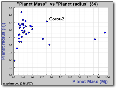
The CoRoT mission announced their second transiting planet today, and it’s a weird one. The new planet has a mass of 3.53 Jupiter masses, a fleeting 1.7429964 day orbit, and a colossal radius. It’s fully 1.43 times larger than Jupiter.

The surface temperature on this planet is likely well above 1500K. Our baseline theoretical models predict that the radius of the planet should be ~1.13 Jupiter radii, which is much smaller than observed. Interestingly, however, if one assumes that a bit more than 1% of the stellar flux is deposited deep in the atmosphere, then the models suggest that the planet could easily be swollen to its observed size.

The surest way to heat up a planet is via forcing from tidal interactions with other, as-yet unknown planets in the system. If that’s what’s going on with CoRoT-exo-2 b, then it’s possible that the perturber can be detected via transit timing. The downloadable systemic console is capable of fitting to transit timing variations in conjunction with the radial velocity data. All that’s needed is a long string of accurate central transit times.

The parent star for CoRoT-exo-2-b is relatively small (0.94 solar radii) which means that the transit is very deep, of order 2.3%. That means good signal to noise. At V=12.6, the star should be optimally suited for differential photometry by observers with small telescopes. With a fresh transit occurring every 41 and a half hours, data will build up quickly. As soon as the coordinates are announced, observers should start bagging transits of this star and submitting their results to Bruce Gary’s Amateur Exoplanet Archive. (See here for a tutorial on using the console to do transit timing analyses.)

The latest on 55 Cancri

Image Source.

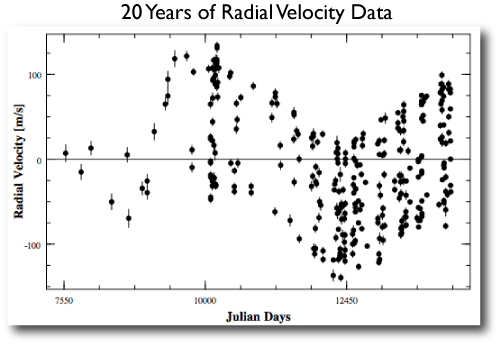
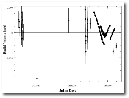
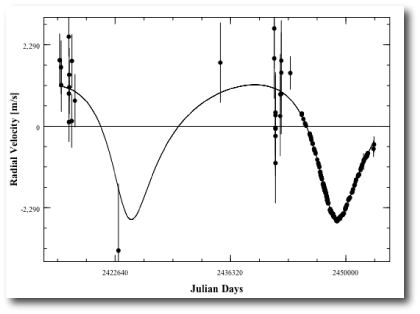
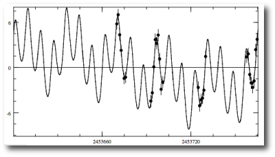
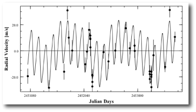
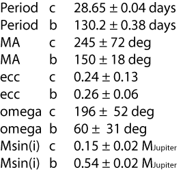
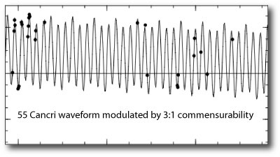
Here’s a development that systemic regulars will find interesting! In a press release today, came announcement of the detection of a fifth planet in the 55 Cancri system (paper here). The new planet has an Msin(i) of 0.144 Jupiter masses, a 260-day orbital period and a low eccentricity. The detection is based on a really amazing set of additions to the Lick and Keck radial velocities:

For background on the 55 Cancri system, check out this oklo.org post from December 2005.

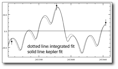
The outer four planets in the 55 Cancri system all have fairly low eccentricities in the new five-planet model. This leads to a diminished importance for planet-planet interactions, but nevertheless, the system does require a fully integrated fit. Deviations between the Keplerian and integrated models arise primarily from the orbital precessions of planets b, c, and e that occur during the long time frame spanned by the radial velocity observations.

Eugenio has added the velocities onto a fully updated version of the downloadable systemic console. The new version of the console adds a wide variety of new features (including dynamical transit timing) that were formerly available only on the unstable distribution. Check it out, and see the latest news on the console change log and the backend discussion forum. Over the next month, we’ll be talking in detail about the new features on the updated console.

Very shortly, a new entries corresponding to the updated 55 Cancri data sets will be added to the “Real Stars” catalog on the systemic backend. I’ll then upload my baseline integrated 5-planet fit to the joint Keck-Lick data set. I’m almost certain that with some computational work, this baseline model can be improved. Such a task is not for the squeamish, however. Obtaining self-consistent 6-body models to the 55 Cancri data set is a formidable computational task for the console. There are 29 parameters to vary (if the Lick, Keck, ELODIE and HET radial velocity data sets are all included). The inner planet orbits every 2.79 days, and the data spans nearly two decades. Fortunately, Hermite integration is now available on the console. Hermite integration speeds things up by roughly a factor of ten in comparison to Runge Kutta integration.

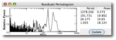
There have been hints of the 260-day planet for a number of years now because it presents a clear peak in the residuals periodogram. After the 2004 announcement of planet “e” in its short-period 2.8 day orbit, Jack Wisdom of MIT circulated a paper that argued against the existence of planet “e”, and simultaneously argued that there was evidence for a 260-day planet in the data available at that time. More recently, a number of very nice fully self consistent fits to the available data have been submitted to the backend (by, e.g., users thiessen, EricFDiaz, and flanker). Their fits all contain both the 2.8 day and the 260-day planets, and happily, are fully consistent with the new system configuration based on the updated velocities. Congratulations, guys!

Interestingly, the best available self-consistent fits to the system indicate that planets b and c do not have any of the 3:1 resonant arguments in libration. It will be interesting to see whether this continues to be the case as the new fits roll into the systemic backend.

Systemic in the Classroom

Image Source.

In our development of the systemic console and the systemic backend, we’ve strived to build a professional-quality tool that can be used by the general public. There’s no better way to get a sense of them planetary discovery process than to participate yourself, and so we’d like to encourage astronomy instructors to fold the systemic console into their curricula.

This link points to a Word format document of a sample homework assignment that makes use of both the console and the systemic backend. We’ve had good success with this particular problem set at UCSC, and it’s currently being implemented at MIT as well. The level has been found to be appropriate to an astrobiology class for science majors. There’s no math prerequisite, so it can also be fully useful for a non-major survey course.

If you’re an astronomy instructor and you’d like to incorporate hands-on planet finding into your course, let me know, and we can set up a fit submission aggregator for your students on the systemic backend.

fit to be timed

Image Source.

One reason why extrasolar planets are so exciting is because they are accessible. You don’t need a Ph.D. or a large laboratory or a space-borne telescope to make an important discovery. There are very few areas in science where such a wide pool of workers can contribute in a fully meaningful way.

On the systemic backend, the focus is largely on planet characterization through the analysis of radial velocity data. At Transitsearch.org, the goal is to provide the information that will allow small telescope observers to discover transiting planets. Transitsearch, however, is mainly a repository for transit predictions. We maintain information about when and where to look, but we fall short when it comes to explaining how to obtain high-precision photometry. There has long been a need for a good end-to-end manual on the art and science of photometric transit detection.

Bruce Gary is an experienced observer of transiting extrasolar planets, and is a member of the XO network, which has had made several discoveries over the past year and a half (see e.g. here). Bruce has written a book, Exoplanet Observing for Amateurs which he’s made available for free in .pdf form.

Bruce has also launched the Amateur Exoplanet Archive (AXA), which is a repository for light curves obtained for known transiting planets. If you get a photometric transit time series of one of the planets, then make sure that you submit it to Bruce’s archive. With all the data in one place, everyone will have easy access for analysis projects.

Transit midpoint times can be measured from individual light curves, and a sequence of midpoint times can be used to improve the characterization of a particular planetary system. To this end, Stefano has extend the .sys file format used by the systemic console to include “transits” data files (which take a .tds suffix, and which are separate from the .vels files that the console has used all along). If you have transit data, it’s simple to implement one of these files for yourself.

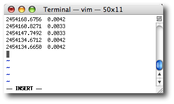
To see how it works, consider the recently discovered transiting planet XO-2. The published radial velocity data for this planet is already bundled with the console. On the AXA site, a total of five transits have already been archived for XO-2. Each of these transits has a measured Heliocentric Julian Date (HJD) for the time of transit midpoint, along with an associated uncertainty. I copied these data into a newly created “X0-2.tds” file in my console’s datafiles folder:

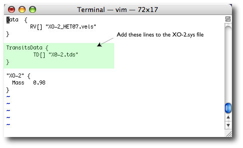
I then added the following lines to the .sys file for the XO-2 system:

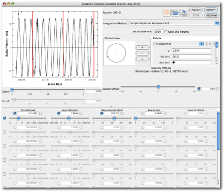
Having done that, I launched the latest (“unstable” Aug. 21, 2007 version) of the systemic console. Stefano has been steadily improving the console’s algorithms, user interface, and performance. If you’ve been working with the standard stable downloadable console, you’ll immediately notice that there’s a lot of new functionality. We’ll be getting a manual out as soon as the much-anticipated Systemic Jr write-up is completed, but in the meantime, there’s a wide variety of resources on the backend that can help you navigate the latest console features.

With the .tds file linked in, the observed transit midpoint times appear as vertical red lines in the radial velocity timeline window. If the “fit transits” option is unchecked, then the console considers only the radial velocity data. If the “fit transits” option is checked, however, then the observed transit times are included as data to be fit. The uncertainties in the transit midpoints can be very small, and so this provides a very strong constraint on the period of the orbit and the time at which the planet crosses the plane containing the line of sight to the Earth. Note that the transit fitting can be done in a fully self-consistent N-body fashion if integration is enabled.

Try it for yourself!

As more transit data is accumulated, it will become possible to do some increasingly sophisticated analyses. Transit timing is potentially a very powerful method for detecting additional, as-yet unseen perturbing bodies in a given system. Objects like Gl 436 b are especially good candidates for this type of approach, and quite a bit of photometric data is being accumulated during the Gl 436 transits.

ƒr3$h R4Ð14£ V3£0(1713$

Image Source.

Eugenio has finished combing through this summer’s literature, and has added twenty newly published radial velocity data sets to both the systemic backend and to the current version of the downloadable systemic console. As a result of his efforts, new or augmented data is now available for the following stars: Cha Ha 8, GJ 317, HD3651, HD5319, HD11506, HD17156, HD37605, HD43691, HD75898, HD80606, HD89744, HD125612, HD132406, HD170469, HD171028, HD231701, NGC2423, NGC4349, HAT-P-3, and TrES-4. As always, the published literature citations for the velocities are contained in the “vels_list.txt” file that comes bundled with the systemic console download. The vels_list.txt file can be indispensible if you want to publish results that use the systemic package as a research tool — indeed, we’re quite excited that researchers are starting to adopt the console in the course of carrying out state-of-the-art research (see, e.g. here.)

There’s quite a bit to explore with these new data sets. Eugenio has had a first look, and included in his recommendations are:

GJ 317: This system (discovered by John Johnson and the California-Carnegie planet search team, preprint here) is only the third red dwarf that’s been found to harbor a Jovian-mass companion. The data shows clear evidence for one planet “b”, with at least 1.2 Jupiter masses and a 693-day orbit, and there’s a strong hint of a second planet in the radial velocity variations. Check it out with the console!

HD 17156: This data comes from a recent paper by the California-Carnegie team. There are radial velocities from both the Keck and the Subaru telescopes, and the signal-to-noise of the orbit is very high.

The data show a ~3 Jupiter-mass planet on a 21.2 day orbit. The orbit is remarkably eccentric for a planet on such a short period, leading to a 25-fold variation in the amount of light received during each trip around the star.

It’ll be interesting to get a weather forecast for this world, and it’s also important to point out that the orientation of the orbit is very well suited for the possibility of observing transits. Periastron is reasonably close to being aligned with the line of sight to Earth, leading to an a-priori transit probability of more than 10%. In the discovery paper, a preliminary transit search is reported, but only about 1/4th of the transit window was ruled out. With a Dec of +71 degrees and a nice situation in the winter sky, this is definitely one for Transitesearch.org’s Finland contingent.

transitsearch dot org

Image Source.

Gl 436 b was the first planet to be detected in transit after the radial velocity detection of the planet itself was publicly announced. Gillon et al.’s discovery shows that the basic strategy of checking known Doppler wobble stars for transits can pay off dramatically, and indeed it’s recharged my interest in keeping transitsearch.org up and running.

Successful transit predictions depend on having accurate ephemerides, which in turn depend on fits to the most recent radial velocities available. The period error in an old fit builds up to the point where the predicted transit window is longer than the orbital period itself. Indeed, relying on a published fit that’s five, six, or even eight years old, is akin to showing up at the 2007 Grammy Awards in a 2001 Escalade.

We’ve thus started the job of making sure that the transitsearch.org candidate tables are as up to date as possible. I’ve committed to spending a bit of time each day checking and updating the master orbit.data and star.data files that are used as input to the cron job that runs every night to update the prediction tables. In each case, we’ll use the most recent published orbital data for a given planet.

In addition, the eighteen known transiting planets have all had their ephemeris tables updated using the latest literature values for the orbital parameters. I got the most of these data from Frederic Pont’s useful summary table, and took the radial velocity half-amplitudes from exoplanet.eu and exoplanets.org. At the moment, the occultations are all treated as central transits by my code, which means that the predicted transit durations will in general be longer than the actual observed events. This discrepancy will be patched shortly, but in the meantime, the predicted transit midpoint times in the ephemeris tables should be extremely accurate for all 18 planets. (See the candidates faq for more information).

We’ve made the decision to base the main transitsearch.org candidates table only on published orbital fits that have appeared in the refereed literature. In many cases, however, one finds a need to go beyond predictions based on published fits. There are two main circumstances under which this can occur. (1) The systemic console provides the ability to obtain fits to all existing radial velocity data for any given system. For many systems, one thus has the opportunity to obtain orbital parameters for the planet that are more accurate than published values that are based on fewer data sets. (2) You may have used the console to locate a candidate planet that is not yet published. If this planet can be observed in transit, then you’ve got dramatic confirmation of your discovery.

Eugenio has written an extension to the bootstrap window of the most recent version of the console that allows anyone to make transit predictions for any planet produced by the console. In an upcoming post, we’ll look in detail at how this new feature works.

Systemic Jr. Fit Drive

Image Source.

A big thank-you to everyone who’s been participating in the drive to characterize and study the catalog of synthetic “Systemic Jr.” planetary systems on the Systemic Backend. There’s now enough data to indicate that the analysis is going to be very informative. We’re looking forward to revealing the properties of the underlying planetary systems that were used to generate the data. In the meantime, we need your help to adequately characterize all 520 systems. Data in need of better characterization are marked by flags:

Our backend server is now swarming with various hard-working software robots that Stefano has assembled. The 100-year stability bot is rousted out of bed and set to work whenever a new fit is submitted. It reports a quick initial assessment of orbital stability. Planetary systems that pass through the 100-year stability screen are then put in a queue to wait for the attentions of the 1000-year stability bots. Systems that make it through 1000 years with less than a 1% change in semi-major axis of their planets are awarded a snazzy green flag:

Occasionally, systems that are in mean-motion resonance can show periodic semi-major axis variations of more than 1% while still remaining indefinitely stable. A resonance bot that will go through the fits and check for these special cases is currently being readied.

Systems that pass the minimum stability requirement are handed to a bootstrap bot which uses the bootstrap method to estimate uncertainties on the planetary orbital parameters for each stable fit. We’re currently running the bootstrap bot under the assumption that the orbits are pure Keplerian ellipses, and so the calculations are usually quite rapid. Very shortly, the error estimates for the parameters in submitted fits to the real systems and the Systemic Jr. systems will be showing up on the back-end data pages.

Finally, an “F-bot” has been activated which performs successive F-tests on submitted multiple-planet systems. Using its results, we’ll have a better idea of when the addition of a planet to a system is warranted.

Bootstrap

Image Source.

Stefano and Eugenio have been making quite a bit of development progress on the downloadable systemic console. A new version of the console (available for beta testing on the systemic backend) is now capable of providing an estimate of the uncertainties on the orbital elements associated with a fit to a particular data set.

Radial velocity data don’t provide an exact determination of planetary orbits. The most obvious shortcoming is that Keplerian orbital fits can’t determine the inclination of the planetary orbits, and so for a given system, we’re only able to measure then mass of the planet multiplied by the sine of the unknown inclination angle. Furthermore, the stellar radial velocity signal created by a planetary system is corrupted by astrophysical noise introduced by the parent star, as well as by noise introduced during the measurement process here on Earth.

Determination of the true uncertainties in a planetary orbital model is a subtle problem (for more detail, see Eric Ford‘s recent work in this area). As a first straightforward step, we’ve implemented the so-called “bootstrap” method of error estimation into the console. The bootstrap works by taking the original data set, and then successively redrawing time + velocity + uncertainties triples from the data with replacement. This procedure creates alternate realizations of the original data set in which some of the original measurements appear more than once, and in which some don’t appear at all. The best-fit parameters obtained by the console are then used as a starting guess to fit the bootstraped data sets. The standard deviations measured from the distributions of orbital elements thus obtained give error estimates for the parameters of the original fit.

The bootstrap routine is menu-accessed, and is simple to use. First, create a fit to a dataset. In the example just below, I’ve fitted to the data for HD 80606:

Once the fit has been polished, the bootstrap can be run. In the default configuration it uses Keplerian fitting and does 100 trials.

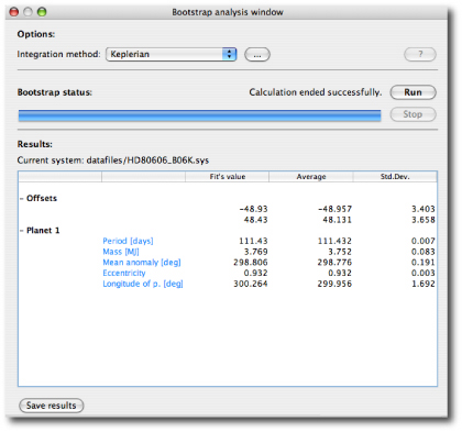
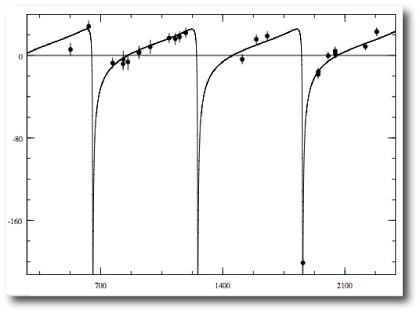
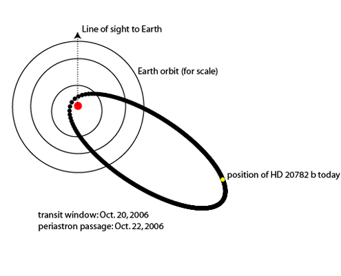
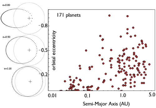
HD 80606 has been observed for nearly 20 orbital periods, and velocities have been obtained at a wide variety of orbital phases. As a result, the orbit is very well constrained. The bootstrap indicates that the uncertainty on the e=0.932 eccentricity is only 0.003. For other systems, such as hd 20782, which also seems to have a high eccentricity:

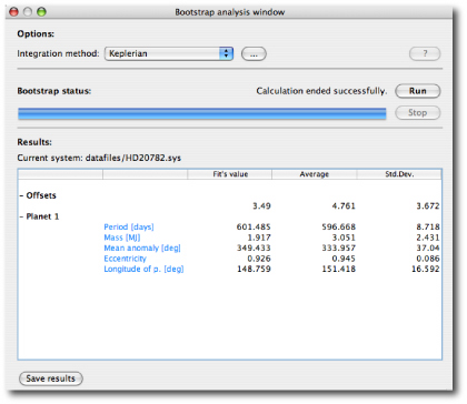
the uncertainty on the parameters is much larger:

Give the routine a try! In upcoming posts, we’ll talk more about how uncertainty estimates will be incorporated into the planetary catalogs on the backend.

The exoplanet prediction market

Image Source.

At first glance, the market capitalization of the Chicago Board Options Exchange, and the list of astronomers active in the field of extrasolar planets would appear to have nothing to do with one another. These two disparate entities are connected, however, by the fact that they’ve both undergone explosive growth over the past decade, and both are continuing to grow. They signify highly significant societal trends.

I think it’s safe to predict that in 25 years, the market for financial derivatives, and the level of economic activity associated with exoplanets will both be far larger than they are now. It’s interesting to ask, will there be an unanticipated co-mingling between the two? And if so, how will it occur?

One very realistic possibility is the development of an exoplanet prediction market, in which securities are issued based on particular fundamental questions involving the distribution of planets in the galaxy. Imagine, for example, that you’re an astronomer planning to devote a large chunk of your career to an all-or-nothing attempt to characterize the terrestrial planet system orbiting Alpha Centauri B. In the presence of a liquid, well-regulated exoplanet prediction market, you could literally (and figuratively) hedge your investment of effort by taking out a short position on a security that pays out on demonstration of an Earth-mass planet orbiting any of the three stars in Alpha Centauri.

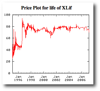
Prediction markets have been adopted in a very wide range of contexts, ranging from opening weekend grosses for big-budget movies, to forecasts of printer sales, to the results of presidential elections. A highly readable overview of these markets by Justin Wolfers (who was featured last week in the New York Times) and Eric Zitzewitz of the University of Pennsylvania is available here as a .pdf file. The ideosphere site contains a wide variety of markets (trading in synthetic currency) and includes securities directly relevant big-picture questions in physics, astronomy and space exploration. Here’s the price chart for the Xlif claim,

which pays out a lump-sum of 100 currency units if the following claim is found to be true:

Evidence of Extraterrestrial Life, fossils, or remains will be found by 12/31/2050. Dead or extinct extraterrestrial Life counts, but contamination by human spacecraft doesn’t count. (Life engineered or created by humans doesn’t count.) The Life must have been at least 10,000 miles from the surface of the Earth. If Earth bacteria have somehow got to another planet and thrived, it counts, as long as the transportation wasn’t by human space activities.

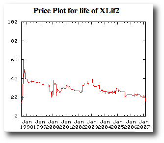
It’s very interesting to compare the bullish current Xlif price quote of 72 with the far more bearish sentiment on Xlif2, which is currently trading at an all-time low of 17,

and which pays out if “extraterrestrial intelligent life is found prior to 2050”, and more specifically,

Terrestrial-origin entities (e.g. colonists, biological constructs, computational constructs) whose predecessors left earth after 1900 do not satisfy this claim. If the intelligence of the ET is not obvious, the primary judging criteria will be either a significant level of technological sophistication (e.g. radio transmitting capability) or conceptual abstraction (e.g. basic mathematical ability). Radio signals received or similar tell-tale signs of intelligence (e.g. archeological discoveries) detected and accepted by scientific consensus as originating from intelligent extraterrestrials would satisfy the claim even if not completely understood by the claim judging date.

Recently, open-source software has been released that makes it straightforward to set up a prediction market. We’ll soon have the world’s first exoplanet stock market up and running right here at oklo.org. In the meantime, feel free to submit specific claims (in the comments section for this post) that might lend themselves to securitization…

Lonely Planet Guide to the Hyades

Image Source.

It’s been a hectic week, and now that it’s February, my New Year’s resolution to write 2-3 posts per week managed to lose its shaky option on my priorities.

Eugenio stopped by my office this afternoon to outline his latest code developments for the console. He’s mostly finished implementing a Bulirsch-Stoer integrator. Once this algorithm is tested and operational, it will produce very significant speed-ups for the fitting and the stability analysis of tough multiple-planet systems such as 55 Cancri and GJ 876. Then it’ll be on to a rollout of the bootstrap method for computing uncertainties for the orbital elements in the planetary fits.

“So did you see the new planet?” he asked.

“Huh?” I hadn’t heard anything about it.

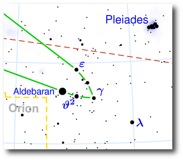
Turns out that Bunei Sato and his collaborators have detected a periodic radial velocity variation for the star Epsilon Tauri. Their preprint is on the Astrophysical Journal’s website, but it doesn’t seem to have hit the preprint server yet. This star is a prominent member of the nearby Hyades cluster, and is easily visible to the naked eye as part of the well-known “V”-shaped asterism near Aldeberan in the sky.

Image Source.

Eps Tau is bright enough to have garnered 40 different names in the Simbad catalog, and it’s now listed in the console menu and on the systemic backend as HD 28305. This is one of the most straightforward radial velocity datasets that you’ll come across, and thus makes a good system for first-time users to fit. A few debonair moves with the downloadable console conjure up a model planet with a period of 594 days, an orbital eccentricity e=0.15, and a minimum mass 7.6 times that of Jupiter:

Epsilon Tauri is one of the four stars in the Hyades that are currently nearing the end of their lives and are evolving through the red giant phase. It’s 14 times larger than the Sun, and it’s luminosity is 97 times the solar value. It weighs in at 2.7 solar masses, making it the most massive star known to harbor a planet.

So what’s the story? The Hyades are a metal-rich cluster. One would naively expect that the supersolar composition of the precursor star-forming giant molecular cloud would have lead to a large fraction of the cluster members harboring readily detectable planets. It’s also true that stars somewhat more massive than the Sun should harbor a higher-than-average fraction of giant planets. Eps Tauri scores on both counts.

[Note: John Johnson‘s thesis work at UC Berkeley and Bunei Sato’s RV survey are both capable of providing observational support for the hypothesis of a positive correlation between the detectable presence of a planet and the mass of the parent star. See talk #1 on the Systemic Resources page for more details.]

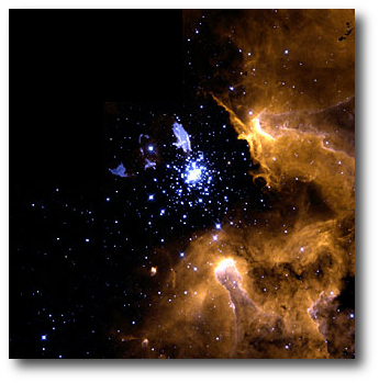
Young Cluster NGC 3603, Source: NASA

It’s important to keep in mind, however, that a cluster environment will have a strong effect on giant planet formation. Currently, the Hyades are 600 million years old, and the cluster has lost a large fraction of its O.G.s to the general galactic field through the process of dynamical escape. If we extrapolate back to the cluster’s early days, we find that the Hyades would have resembled the Pleiades 500 million years ago, and would have looked like the Orion Nebular Cluster during the first few million years of its existence.

The UV radiation environment in the original Hyades cluster was fierce. The protostellar disks of the individual Hyads were likely photoevaporated before the growing planetary cores were able to reach the runaway gas accretion phase that gives rise to Jupiter-mass planets (see our paper on this topic). When we get the full inventory of planets in the Hyades, I think we’ll find plenty of Neptunes and terrestrial planets, but almost nothing in the Jovian range. Indeed, work by Bill Cochran and the Texas RV group has demonstrated that the Hyades are generally deficient in massive planets.

My guess is that Epsilon Tauri b is an example of a planet that formed through the gravitational instability mechanism. Gravitational instability should generally produce more massive planets (e.g. HIP 75458 b, and HD 168443 b and c) and its efficacy will be little-affected by UV radiation from neighboring stars. It likely occurs once per every several hundred stars that are formed, and so it’s perfectly reasonable that there’s one star in the Hyades that has a planet formed via the GI mechanism.

For more information, this series: 1, 2, 3, 4, 5, 6, and 7
of oklo posts compares and contrasts the gravitational instability and core accretion theories for giant planet formation.

a bunch of cool new stuff

Image Source.

Stefano and Eugenio have both been working hard on the systemic console and backend, and as a result of their efforts, we’re now able to roll out a number of new features.

The backend now features a systemic wiki in which users can collaborate on a wide variety of writing projects related to systemic in particular and extrasolar planets in general. Features include discussion pages for individual systems, the framework for a comprehensive console and backend manual, and an exoplanetary news wire. Our first news service is being provided by Mike Valdez, who combs astro-ph every day and extracts any new preprints that are germane to the those interested in exoplanets. Stefano wrote the code from scratch, so there are endless possibilites for customization. Give it a try.

On the console front, Eugenio has aggregated a uniform listing of the literature sources of all of the radial velocity data sets provided by the console. This information is in a file vels_list.txt, which is now included in the systemic.zip package. If you are using the console for scientific research that you intend to publish, it’s now a snap to get the correct citations for any of the individual systems included on the console.

Many users have expressed interest in what our own solar system would look like to a dedicated radial velocity observer on another star. Eugenio has put together an expansion pack that contains 17 manufactured data sets based on the Solar System. A second expansion pack contains an analogous set of manufactured data sets for various plausible configurations of planets orbiting Alpha Centauri A and B. Both are available on the downloads page for the downloadable systemic console.

Check it out!

mp3s of the spheres

Image Source.

New users are still streaming into oklo.org. If you’re a first-time visitor, welcome aboard. You’ll find information that you need to get started in this post from several days ago.

The EZ-2-install downloadable systemic console is the primary software tool that we provide for analyzing data from extrasolar planetary systems. The tutorials 1,2, and 3 are the best way to learn how to use the console. Over the past few months, we’ve been adding a range of new capabilities that go beyond the features described in the tutorials and which improve the overall utility of the software. We’ll be explaining how these new features work in upcoming posts, and for our black-belt users, we’re also putting the finishing touches on a comprehensive technical manual.

When we designed the console, our main goals were to produce a scientifically valuable tool, while at the same time make something that’s fun and easy to use. Early on, we settled on the analogy with a sound mixing board, in which different input signals (planets) are combined to make a composite signal.

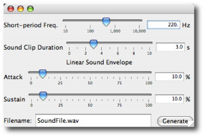
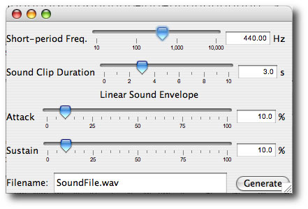
We’ve pushed the audio analogy further by adding a “sonify” button to the console. When sonification is activated, you can turn the stellar radial velocity curve into an actual audible waveform. If you create a system with several or more planets, these waveforms can develop some very bizarre sounds. From a practical standpoint, one can often tell whether a planetary system is stable by listening to the corresponding audio signal. Alternately, the console can be used as a nonlinear digital synthesizer to create a very wide variety of tones.

Here are links (one, and two) to past posts that discuss the sonification button in more detail. If you come up with some useful sounds, then by all means upload the corresponding planetary configurations to the systemic back-end.

Armchair Planet Hunting

Image Source.

The Associated Press just published an article on how the Internet has facilitated an increasing number of collaborations between amateur and professional astronomers. The systemic project is one focus of the AP piece, and we’re seeing a jump in traffic as a result. If you are a first-time visitor to the site, welcome aboard!

There are several ways that you can use and participate in systemic. Our project home page is a weblog (updated fairly frequently) that gives an insider’s perspective on the latest developments and discoveries in the fast-moving fields of extrasolar planets and solar-system exploration. We write for a target audience of non-astronomers who are interested in astronomy. To get a flavor for the blog, keep reading the posts below, or have a look at a few of our past articles, such as our take on last Summer’s big “is Pluto a planet debate”, our exploration of what planets and galaxies really look like, or our series [1, 2, 3, 4] on the feasibility of detecting habitable terrestrial planets in the Alpha Centauri System.

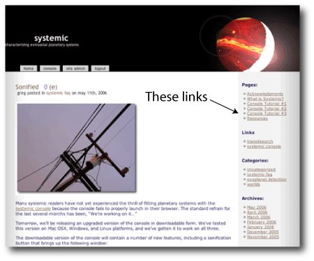
You should see a set of links just to your right:

These links give you information that you can use to start participating in the actual discovery and characterization of extrasolar planets. (Despite the fact that we’re rocket scientists, we’ve been unable to consistently sweet-talk Microsoft IE into correctly displaying our site. On some versions of IE, you may have to scroll all the way down to the bottom of this page to see the links). The Downloadable Systemic Console is our Java-based software package that allows you to work with extrasolar planet data. The Systemic Backend is a collaborative environment that has the look and functionality of a social networking site. Registration and participation are free. The nearest well-characterized extrasolar planets (GJ 876 b, c and d) are 14.65 light years away, and so the news of useful modern innovations such as pop-ups and spyware hasn’t had time to propagate to those far-distant worlds. Hence the systemic backend is completely free of annoying ads!

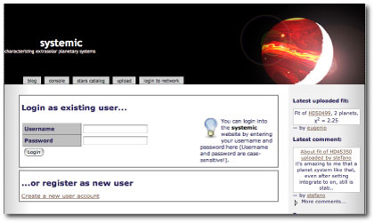
One final note: there are two separate channels for registration on systemic. The first, accessed through the “login” tab on the site header above, is part of the WordPress package that runs the blog. Registration on the blog allows you to comment on our frontend posts. The second, accessed through the “backend” tab on the site header or the link to the right, gives you access to the collaborative php-based environment that constitutes the systemic backend. You can register for either or both, and you don’t need to give your real name or any real-world identifying information other than an e-mail address.

Tune in regularly for more news and updates.

year 2.0

Image Source.

As of tomorrow, oklo.org will have been on the air for one year. We’re pleased with the response that we’ve gotten thus far, and we’re looking forward to rapid progress during year two. A big thank-you is definitely in order to everyone who’s either worked on the site or made regular visits or participated in the ongoing collaborative research!

In recent weeks, the user base on the systemic back-end has grown substantially, and we’ve been pushing the limits of what our ISP is geared to provide. Bluehost provides a very cost-effective package for hosting weblogs and running small-scale sites, but it’s become abundantly clear that one can’t expect to run a web 2.0 startup for $6.95 per month. At that level of expenditure, we’ve been limited to the use of 20% of one processor with a maximum job length of 60 seconds. Stefano has stretched our ration with clever use of cron command, but nevertheless,

has become a refrain tiresomely familiar to backend users, and our attempts over the past week to shift the backend to alternate stop-gap servers have been thwarted by various software incompatabilities.

I’m thus very happy to report that an order has been placed for a dedicated server that will obliterate the current problems. It will be located in downtown Santa Cruz on a high-speed T3 line. We should have everything up and running on it within 2 weeks. It’s spec’d to run the full systemic simulation, the new connection is ready to handle a hoped-for shout-out from boing-boing or slashdot, and the joint package should deliver a much more satisfying end-user experience.

In the meantime, however, keep sending in those fits. Neither sleet, nor snow, nor server overloads shall… We’re very eager to build up a solid distribution of fits for Systemic Junior.

Viewed from afar (Challenge 004)

Image Source.

The fourth systemic challenge turned out to be somewhat less challenging than the first three. Quite a few entrants figured out that the data-set corresponds to our own solar system. Among a large number of excellent models, Mark Kilner turned in the fit with the lowest chi-square: 1.0401. In addition to Jupiter, Saturn, Earth, and Venus, he topped off his system with a spurious Mercury-mass planet in a 5.62 day orbit, which allowed him to take the prize. Nice one, Mark!

Eugenio created the challenge 004 synthetic data set after a conversation in which we decided that it’ll soon be feasible to push the precision of the radial velocity method down to an instrumental error of 0.1 m/s. Even more optimistically, we assumed that the Sun, viewed from afar, exhibits negligible radial velocity noise (more on that soon).

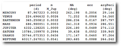
Our Solar System, expressed in the Jacobi orbital elements used by the console, is given by:

The true three-dimensional model that Eugenio actually integrated to produce the synthetic data set also includes the correct values for the planetary inclinations and nodes. Because of the sin(i) degeneracy for Keplerian orbits, the current version of the downloadable systemic console does not include the inclinations and nodes as fitting parameters.

The synthetic data set was created with the KeckTAC program, which mimics realistic observing strategies. In an all-out effort on a particular star, one would combine repeated individual observations to get a composite observation that averages over the effect of short-period oscillations (p-modes) of the star itself. This is the strategy that is being currently used by the Swiss team in their campaigns on stars such as HD 69830 and HD 160691. In the challenge004 dataset, there are 1171 radial velocity measurements spread out over 24 years.

Eugenio describes the procedure he used to fit the data:

The periodogram (and the data) shows Jupiter clearly. Saturn appears as a trend, but the periodogram of the residuals after fitting Jupiter gives a good guess for Saturn’s period. After removing Saturn, Earth pops out in the residuals periodogram. I did not find it easy to fit Jupiter, Saturn, and Earth, but after succeeding, Venus very clearly appears in the residuals. I kept on fooling around with the 4-planet fit to see if there was any chance of finding Mars even though the RMS was telling me that 4 planets was the best that I would likely do. I was hoping that N would be large enough to let me get Mars, but I was not able to see a (significant) signal in the residuals periodogram. If anything, Mercury seemed to be more easily detectable. However, after fooling around with the eccentricities of Saturn, Earth, and Venus, the (weak) signal for Mercury disappeared.

Image Source.

With the contests wrapped up, we’re now in the business of getting the fits completed for the Systemic Jr. data set. Eugenio recently incorporated an F-test module into the console, which can be used to determine whether the addition of a planet is warranted. We’ll have a post up shortly that explains in detail how this works. In the meantime, see the discussion on the backend, or download a new console and give its new modules a whirl.

Apsidal

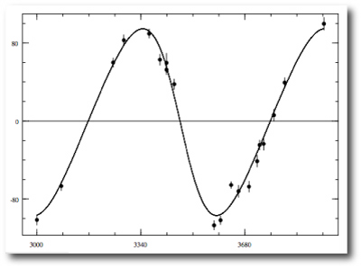
In 1999, Upsilon Andromedae burst onto the international scene with the first known multiple-planet system orbiting a sunlike star. Eight years later, we know of twenty-odd additional multiple-planet systems, but Ups And remains a marquee draw. No other system evokes quite its exotic panache. No other extrasolar planets have garnered names that have stuck.

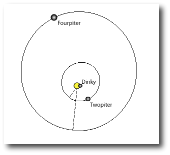
High in the cold and toxic atmosphere of Fourpiter, Upsilon Andromedae shines with a brilliance more dazzling than the Sun. Twopiter is occasionally visible as a small disk which, near conjunction, subtends about one-tenth the size of the full Moon in Earth’s sky. Dinky, which lies about four times closer to the star than Mercury’s distance to our Sun is lost in the glare.

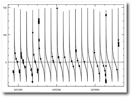
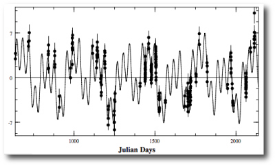
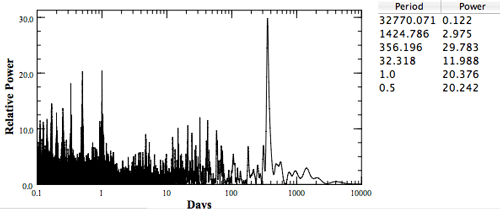
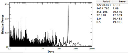
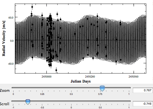
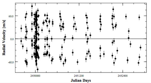
To date, Upsilon Andromedae has accumulated a total of 432 published radial velocities from four different telescopes. The full aggregate of data is available on the downloadable systemic console as upsand_4datasets_B06L. The velocities span nearly two decades, during which the inner planet, “Dinky”, has executed well over 1000 orbits.

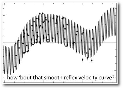
In earlier versions of the console, use of the zoom slider on an extensive data set would reveal a badly undersampled radial velocity curve at high magnification. Eugenio’s latest console release has addressed this problem, however, and the radial velocity model curve now plots smoothly even with the zoom slider pulled all the way to the right.

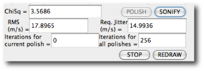
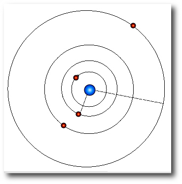
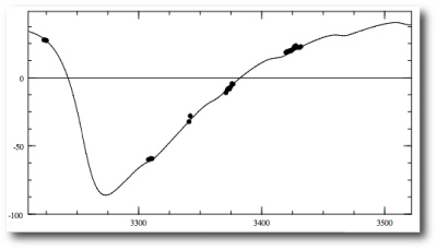
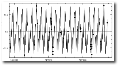
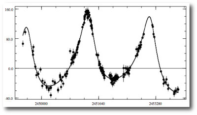
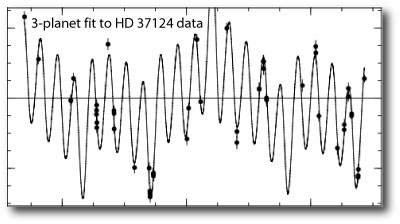
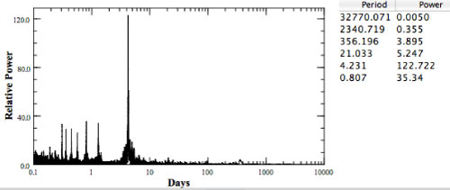
It’s interesting to look at the best radial velocity fit to all four data sets. The planets are very well separated in frequency space, and so it’s a straightforward exercise to converge on the standard 3-planet fit. Upsilon Andromedae itself is a little too hot (6200K) to be an ideal radial velocity target star, and so the chi-square for the best fit to the system is above three, with a likely stellar jitter of a bit more than 14 meters per second. If Ups And were a slightly cooler, slightly older star, we’d potentially be able to get a much more precise snapshot of the planet-planet interactions. (In that Department, however, there’s always 55 Cancri.)

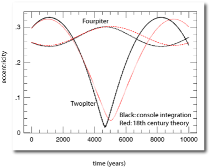
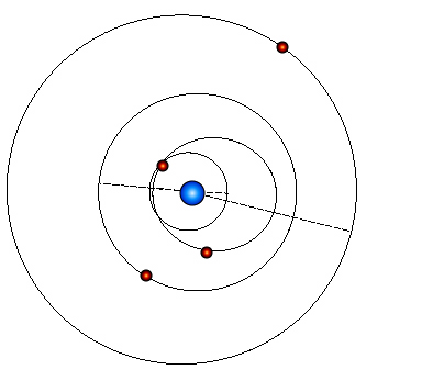
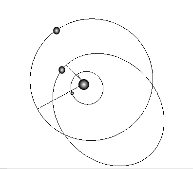
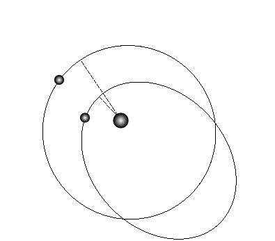
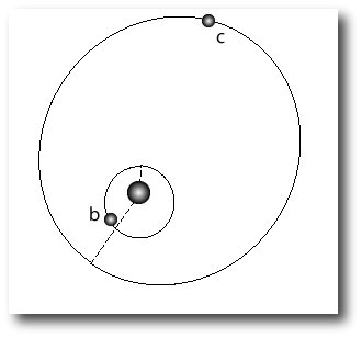
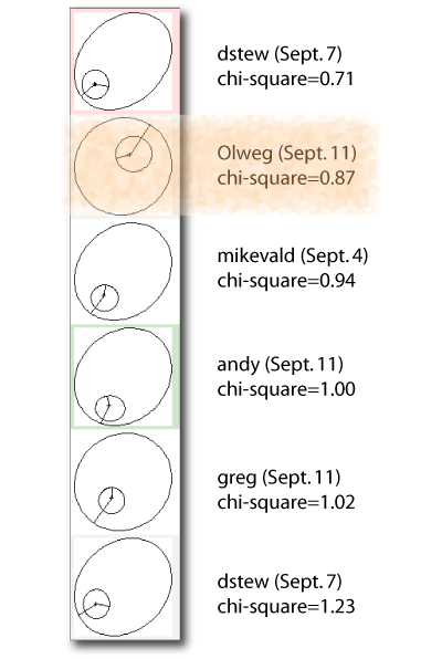
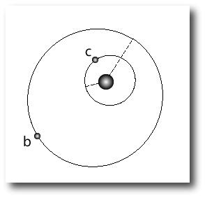
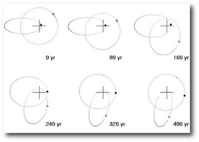
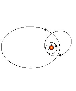
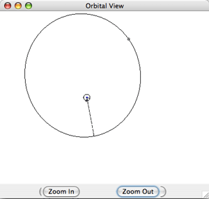
The best fit shows that the apsidal lines of the two outer planets are currently separated by 30 degrees, and are executing very wide librations about alignment. This configuration continues to support the formation theory advanced two years ago by Eric Ford and his collaborators. They hypothesize that Ups And originally had four giant planets instead of the three that we detect now. The outer two (Fourpiter and, uh, “Outtathere”) suffered a close encounter followed by an ejection of Outtathere. Fourpiter, being the heavier body, was left with an eccentric orbit. Now, 2.5 billion years later, the memory of this disaster is retained as the system returns every ~8,000 years to the eccentricity configuration that existed just after the disaster.

Systemic Jr.

Image Source.

The activity this week has all been under the hood, and as a result, the systemic front-end has languished without news. Apologies for that! A slew of updates are on the spike.

Stefano is now officially on the roster at Oklo HQ, and we’re very happy to have him here. The atmosphere is caffeine-fueled startup. He’s already implemented numerous updates and improvements to the systemic backend which, when coupled with Eugenio’s progress on the console, put our web 2.0 story into high gear.

There were a number of times last week when the oklo.org site was temporarily unavailable. Our ISP restricts us to no more than 20% of a full processor load, and exceeding this causes the site to shut down for 5 minutes. We’re now in the process of temporarily mirroring the backend on a machine at Lick Observatory, and quite soon we’ll have a dedicated server up and running.

The systemic Junior datasets have now been added to the downloadable systemic console. Eugenio writes (see the backend discussion forum for the full description):

Systemic Jr. is now included in systemic.zip. You will see two drop down boxes in the upper right region of the main console. One is used to choose a real star system, while the other one is used to pick a Systemic Jr. system. Note that while both boxes are enabled, only one data set is actually selected. In the systemic directory, you will see two new items: “sysjrSystems.txt” and the directory “sysjrdatafiles.” These hold the information needed for Systemic Jr.

As soon as the Lick Observatory server is online, the backend will be able to accept fits to the Systemic Jr. data sets. In the meantime, please save your fits on your local machine. Some of the Systemic Jr. systems may seem familiar. It’s best however, if all of the datasets are approached without a pre-conceived notion of what might be generating them. Once the Systemic Jr. data sets have been fitted, we’ll be able to do a very interesting analysis which will give us some much-wanted information about the nature of the galactic planetary census.

Threaded console available!

Image Source.

This weekend, Eugenio posted an updated version of the downloadable systemic console. The Java code in this version is fully multithreaded, which means that we’re finally able to provide the much-needed and much-requested “stop” button.

For previous console releases, clicking multi-parameter minimization — “polish” — with integration enabled would often cause the console to effectively freeze as the computer worked it’s way through an exceedingly long bout of computation. With the new version, progress is indicated both by a graphical redrawing of the fit, and by a running tally of the number of Levenberg-Marquardt iterations that have been completed. If things appear to be progressing too slowly, it’s now possible to abort to the latest model state by pressing the stop button.

A “back” button will be activated shortly, which will allow you to step backward through your work to revisit earlier model configurations in the session. These features should significantly improve the overall usability of the console.

Another area where progress has been rapid is in the stability checker. Eugenio has put a lot of detailed information on this new functionality on the general discussion section of the backend. In short, the stability checker can now be used as a full fledged integrator which can write time series data to user-specified files. In a post that will go up shortly, we’ll look at how the stability checker can be used to answer some interesting dynamical questions.

Systemic Jr. is also just about ready to go. Assuming that there’s no unforseen snags, we’re looking to launch it on Nov. 1 (next week). In the meantime, download a fresh console, and give the new features a spin.

challenge 4

Image Source.

Eugenio has put the fourth (and final) systemic challenge system on the downloadable systemic console. This dataset is somewhat easier to decipher than the first and second challenges, which were rather esoteric in their planetary configurations. We hope that you’ll find that this one’s a little more down to Earth. I’d like to have your entries in by Oct 31, 23:59 UT. As with our previous three contests, Sky and Telescope is awarding a Star Atlas to the person who achieves the best model of the system.

For this system, it’s likely possible to drive the chi-square arbitrarily close to unity by successively adding spurious, very low-mass planets that act to soak up random noise in the data. We’re currently working on incorporating some standard statistical test utilities into the console which will make it easier to determine whether adding an extra planet is truly necessary. (This will be the topic of an upcoming post, and see the comment thread on Sunday’s post.) For this contest, however, if there are multiple submissions with reduced chi-square near unity, then the prize will be awarded to the fit that also gets the total number of planets in the underlying model correct.

If you haven’t downloaded the console recently, we’re encouraging you to grab a fresh copy. A number of improvements have been added, and there are also a number of additional radial velocity data sets that have been added in recent weeks. Eugenio has been posting a running commentary on the backend describing the console improvements. We’re also putting the final touches on the Systemic Jr. datasets, which we’re hoping to release at the end of next week.

As a result of some articles in the press and on the Internet, we’ve been continuing to see a large increase in the oklo user base. If you’re visiting the site for the first time, you’ll find information about the project and about our goals on the links to the right. Welcome aboard!

1:2:4

Image Source.

The third Systemic Challenge closed to entries on Friday, and I’ve gone through and evaluated the submitted fits. The results were very encouraging. Eight out of twenty-five submissions corresponded to both the correct orbital configuration and the correct number of planets in the underlying dynamical model.

For challenge 003, we looked to our own solar system for inspiration, and tapped the four Gallilean satellites of Jupiter. Eugenio writes:

The system is a scaled-up version of Jupiter and the four Galilean satellites. To generate the model, I first set the central mass to 1 solar mass. The (astrocentric) period of Callisto was set to 365.25 days, and I required that the mass and (astrocentric) period ratios in the system would remain the same. Here’s the resulting model (using Jacobi elements, with i~88 deg):

The Challenge 003 System
Parameter “Io” “Europa” “Ganymede” “Callisto”
Period (days) 38.77079 77.77920 156.65300 365.42094
Mass (Jupiters) 0.04926 0.02646 0.08175 0.05936
Mean Anomaly (deg) 99.453 50.772 285.591 47.538
eccentricity 0.003989 0.009792 0.001935 0.007547
omega (deg) 31.229 205.427 303.460 359.879

Among the eight entries that got both the total number of planets and their periods correct, there was a fair amount of variation among fits that had nearly equivalent values for the chi-square statistic. Chuck Smith (among others) turned in a configuration that bears a very strong resemblance to the actual input system. The four planets in his fit all have nearly circular orbits:

and the resulting radial velocity curve does a very good job of running through the data, with a chi-square value for the integrated fit equal to 1.1005:

A number of other users turned in very similar configurations.

Because of random measurement errors in the data, the true underlying planetary configuration will not necessarily provide the best fit to a given set of radial velocity observations. Often, a better fit can be found for a configuration that is different from the system that generated the data. Steve Undy, for example, achieved a slightly lower chi-square value for his fit by giving a very significant eccentricity to his “Europa”:

The winner of the contest, however, was Eric Diaz, who submitted a 6-planet fit that achieves an integrated chi-square value of 1.04. In addition to the four planets that are actually present in the model, Eric added small planets with periods of 1.06 days and 18.11 days. These objects soaked up some of the residual noise in the fit, allowing for a lower chi-square value, and a copy of the Sky and Telescope star atlas. Nice job Eric!

The contest raises some interesting issues. First, at what point should one stop adding planets to a fit? The chi-square statistic penalizes the inclusion of additional free parameters in a fit, but it’s clear that chi-square can nearly always be lowered by adding additional small bodies to the fit. Second, its very encouraging to see that subtle, but substantially non-interacting systems can be pulled out of radial velocity data sets. In this system, the masses of the planets are small enough so that their dynamical interactions with eachother are not significant over the time-frame that the system is observed. This is in stark contrast to systems such as GJ 876 and 55 Cancri where it is vital to take interactions into account (by fitting with the integrate button clicked on). Finally, I think that we’ll soon see examples of the 1:2:4 Laplace resonance as competitive fits within the existing catalog of radial velocity data sets on the systemic backend.

Gamma Cephei

Image Source.

Guillermo Torres of the CfA recently posted an interesting article on astro-ph in which he takes a detailed look at the planet-bearing binary star system Gamma Cephei.

Gamma Cephei has a long history in the planet-hunting community. In 1988, Campbell, Walker and Yang published radial velocity measurements which show that Gamma Cephei harbors a dim stellar-mass companion with a period of decades. More provocatively, they also noted that the star’s radial velocity curve shows a periodicity consistent with the presence of a Jupiter-mass object in a ~2.5 year orbit around the primary star. In a 1992 paper, however, they adopted a cautious interpretation of their dataset, and argued that the observed variations were likely due to line-profile distortions caused by spots on the stellar surface. From their abstract:

In 1988 Gamma Cep was reported as a single-line, long-period spectroscopic binary with short-term periodic (P = 2.7 yr) residuals which might be caused by a Jupiter-mass companion. Eleven years of data now give a 2.52 yr (K = 27 m/s) period and an indeterminate spectroscopic binary period of not less than 30 yr. While binary motion induced by a Jupiter-mass companion could still explain the periodic residuals, Gamma Cep is almost certainly a velocity variable yellow giant because both the spetrum and (R – I) color indices are typical of luminosity class III. T eff and the trigonometric parallax give 5.8 solar radii independently.

In October 1995, 51 Peg b was announced, and exoplanet research was off to the races. The Walker team, with their futuristic RV surveys had seemingly come close to success, but had not managed to snag the cigar.

In the Fall of 2002, however, the planetary interpretation for the Gamma Cephei radial velocity variations was revived by Hatzes et al., who used McDonald Observatory to extend the data set. They showed that the 2.5 year signal has stayed coherent over two decades, thus effectively ruling out starspots or other stellar activity as the culprit. The planet clearly exists.

Aside from providing a pyrrhic victory for the Walker team, the Gamma Cephei planet is a remarkable discovery in its own right. Its presence showed that gas giants can form in relatively long-period orbits around binary stars of moderate period. In their discovery paper, Hatzes et al. assumed that the binary companion orbits with a period of 57 years, but other estimates varied widely. Walker et al. (1992), for example, adopted 29.9 years, whereas Griffin (2002) use 66 years. The mystery is strengthened by the fact that to date, the companion star has never been seen directly.

The details of the orbit of the binary star are of considerable interest. For configurations where the periastron approach is relatively close, simulations show that the star-planet-star configuration can easily be dynamically unstable.

In his new article, Torres methodically collects all of the available information on the star, and shows that the binary companion to Gamma Cephei has a 66.8 +/- 1.4 year period, an eccentricity of e=0.4085 +/- 0.0065, and a mass of 0.362 +/- 0.022 solar masses. The orbital separation thus lies at the high end of the previous estimates, and renders the stability situation for the system considerably less problematic.

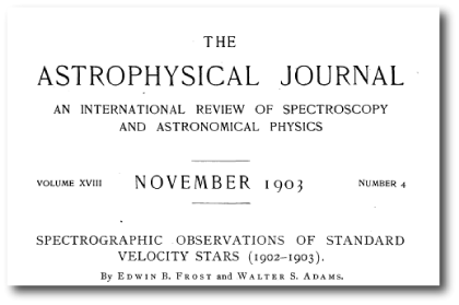
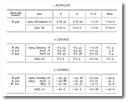
We’re stoked about the Torres paper because it provides references to some truly ancient radial velocities, dating all the way back to a compendium published by Frost and Adams in 1903:

who report 3 measurements made at the University of Chicago’s Yerkes Observatory:

Eugenio has tracked down the various references in the Torres paper, and has recently added all of the available old-school RV’s for Gamma Cephei to the downloadable console. You can access the full dataset by clicking on “GammaCephei_old”:

It’s straightforward to manually adjust the offset sliders to put the radial velocities on a rough baseline. You can then build a rough binary star fit with the sliders, followed by repeated clicking on the Levenberg-Marquardt polish button, with the five orbital elements and the five velocity offsets as free parameters. This gives an Msin(i)=386 Jupiter masses, a period of 24,420 days, and an eccentricity, e=0.4112. Try it! The values that you’ll derive are in excellent agreement with the Torres solution:

With the binary fitted out, try zooming in on the more recent data from the past 10-20 years. You’ll see that the modulation of the radial velocity curve arising from the planet is faintly visible even to the eye. It’s interesting to go in and find the best-fit planetary model…

Follow Ups And other items…

Image Source.

It’s very gratifying to see an increasing number of people logging in to the Systemic Backend, and downloading the console. We’ve also been getting a lot of good feedback from users, which we’ll be incorporating into updated versions of the software.

Several people have noted that the backend is currently assigning chi-square values of zero to uploaded fits! We’re highly aware of this problem, and it likely stems from the fact that we may be exceeding our CPU allocation at our ISP. The back-end code integrates all submitted fits to verify the chi-square statistic for purposes of ranking. For submitted systems with long time baselines and short-period planets, these calculations can wind up being fairly expensive. We’ll let you know as soon as this issue gets resolved. In the meantime, it’s fine to submit fits, but if you get a good one, please save a copy in your own fits directory for the time being.

We’ve been getting a lot of entries for the Challenge 003 system. At the end of this week, I’ll tally up the results, so if you’ve got a fit to submit, go ahead and send ‘er in (using the e-mail address listed on the web-page given in the print version of the October Sky and Telescope). It’s fine to submit multiple fits — I’ll use your best one to determine the final ranking. The challenge 003 system represents an interesting dynamical configuration of a type not yet observed for planets in the wild, and so it’ll be very interesting to see what people pull out. Look for Challenge 004 to appear this weekend on the downloadable console, and shortly thereafter, warm up those processors for the advent of the 100 star Systemic Jr. release.

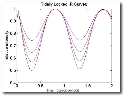
Yesterday’s post is generating an interesting and vigorous discussion thread. Jonathan Langton and I were hopeful yesterday that his benchmark Cassini-State 1 simulation might show an appropriately asymmetric light curve when viewed from lines of sight inclined to the planetary equator (as is the case for the Ups And observations). Frustratingly, however, when the model light curves are actually computed, they wind up drearily sinusoidal, and the phase offset is independant of viewing inclination:

We’re holding out hope, though, for Cassini-State 2. In that case, there are two angles to vary (the orientation of the pole in the orbital plane, and the viewing inclination) and so it may well be possible to dredge up a good fit to the data. After-the-fact parameter tweaking, however, is highly unsatisfactory! I’m looking very much forward to seeing more data sets like Ups And’s. In particular, HD 189733, should give a very nice full-phase curve, and further down the line HD 80606 should be even more interesting.

stability analysis

Rayleigh Taylor fingers

Image Source.

If you’re spending time on the collaborative systemic backend, you’ll know from the discussion threads that Eugenio has been making rapid progress on the downloadable console. He’s in the process of converting the code from a single-thread version to a fully multi-threaded package. Threading is important. It will allow the console to be gracefully reset in the event that a Levenberg-Marquardt polish takes more time than you bargained for, and it will allow for a variety of on-the-fly diagnostics regarding what’s going on under the hood.

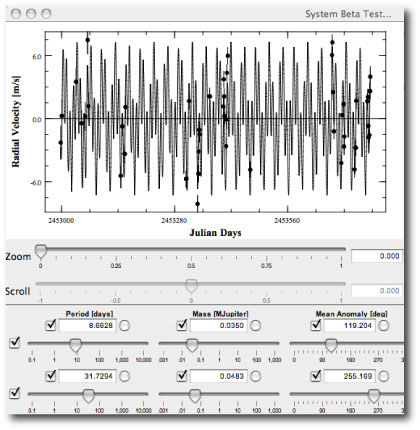
The latest version of the downloadable console now contains a multi-threaded orbital stability checker. To see it in action, download a fresh console (making sure to save your old systemic directory if you have built up a library of fits that you want to keep). I pulled up the HD 69830 dataset and quickly worked up a three-Neptune fit that is very similar to the fit reported by the Geneva team in their discovery paper.

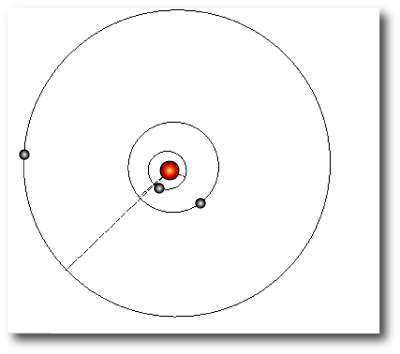
The two outer planets are roughly similar in mass to Neptune, while the inner planet, with a period of 8.66 days is somewhat less massive. It’s not immediately clear from looking at the orbital configuration:

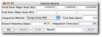
that this planetary troika is gonna get along to go along. A stability check is definitely in order. Clicking on the button for the long-term stability module:

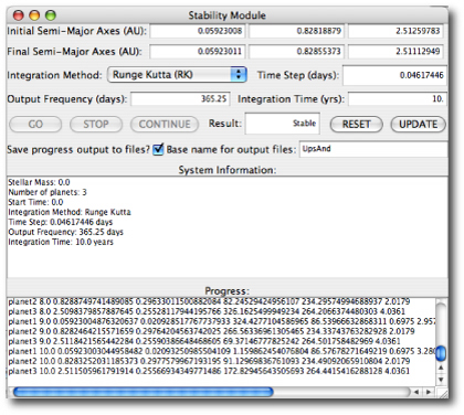
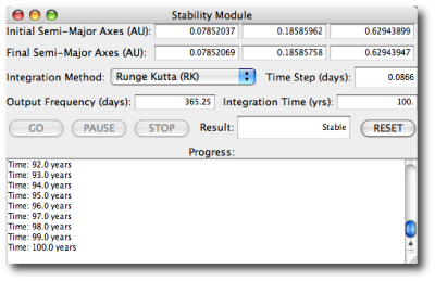
brings up a dialog window that you can use to control the stability integration. You specify the maximum timestep duration, the output frequency, and the integration duration and press go. At present, the console implements only a 4th/5th order Runge-Kutta integrator, but we’ll soon supply faster algorithms, including a Wisdom-Holman symplectic map:

For this example, I specified a short 100-year integration (4200 inner planet orbits). This is enough to see whether the system is wildly unstable, but for a more diagnostic check, one would generally like to look at a longer duration (100,000 inner planet orbits, say).

In this first implementation, a system is deemed “stable” if the semi-major axes of all the planets remain constant to within 1% of their initial values during the course of the integration. There are, of course, stable systems (such as a librating, equal-mass 1:1 resonance configuration) where larger semi-axis variations occur, but if semi-major axes vary by more than 1%, it means that considerable orbital energy is being traded back and forth, and the long-term prognosis is not good.

This HD 69830 3-planet fit easily lasts for 100 years. Nevertheless, as noted in the discovery paper, longer-term integrations show that the system is very close to the edge of stability.

I’m still working on the promised post about trojan planets. Look for it tomorrow!

And inside the second envelope…

Image Source.

First, a thank-you to everyone who submitted a fit to the second systemic challenge. I just loaded all the fits into the console and evaluated the chi-squares (with integration turned on). Jose Fernandes, of Lisbon, Portugal, submitted the winner, and will be receiving the $149.99 sky atlas from Sky and Telescope.

Jose’s fit has a reduced chi-square statistic of 3.94, and is comprised of three planets:

The outer two bodies have masses 1.58 and 0.5 times that of Jupiter, with eccentricities of 0.58 and 0.14. They share a common period of 362 days. The fit also has a tiny inner planet with a mass just under 3% that of Jupiter and a period of 50 days. This little guy improves the fit by wriggling the radial velocity curve up and down to statistically grab more points.

The system that actually generated the data was quite similar:

There are two equal-mass planets with masses 1.04 times that of Jupiter, with eccentricities of 0.7 and 0.2. They share a common period of 365 days. The 50-day planet in the winning fit was spurious, as is often the case when a model planet has a mass that is far smaller than its companions.

This system is an example of a one-to-one eccentric resonance. It is based on a system that was discovered by UCSC physics student Albert Briseno in one of the simulations that he ran for his undergraduate thesis, and it was formed as the result of an instability in a system that originally contained more planets. The system experienced a severe dynamical interaction, which led to a series of ejections. After the last ejection, two planets remained. They share a common orbital period, and gradually trade their eccentricity back and forth. Their interaction gives a strong non-Keplerian component to the resulting radial velocity curve for the star, which makes this a tricky system to fit. While the system might seem absurdly exotic, it’s recently been suggested by Gozdziewski and Konacki that HD 82943 and HD 128311 might have their planets in this configuration (you can of course try investigating this hypothesis for yourself with the console). Their paper is here.

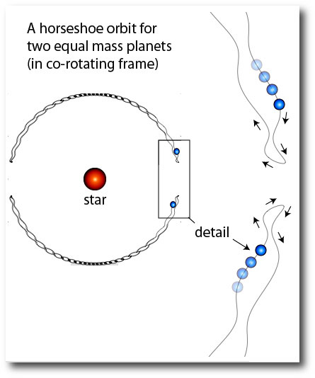
The challenge 002 system is an example of a general class of co-orbital configurations in which the two bodies constitute a retrograde double planet. If you stand on the surface of either world, the other planet appears to be making a slow retrograde orbit around your moving vantage as the libration cycle unfolds over several hundred orbits.

In tomorrow’s post, we’ll stay on the topic of co-orbital planets, and look at some interesting new work by Eric Ford on the possibility that we might soon be able to observe planets in Trojan configurations. Two planets in a Trojan orbit librate around the points of an equilateral triangle in the rotating frame. Indeed, when such an arrangement occurs, it’s possible that a particularly interesting dataset might have the capacity to launch a thousand fits.

[For more about 1:1 resonances, see this post and this post. For a discussion about the audio wave forms that they produce, see this post.]

CfA

Image Source.

Back from a great visit to the Harvard CfA. The exoplanet research effort out there is amazingly comprehensive, and I soaked up a whole range of interesting news items to report. A slew of posts are in the works.

I’ve uploaded my colloquium talk in (1) Apple Keynote format (harvard.key.tar.gz) , (2) Powerpoint format (harvard.ppt.tar.gz), and (3) as a set of .pdfs. The talk was built in Keynote, and thus will look best in that format. Note that the Keynote and Powerpoint files are both quite large (~58MB compressed, ~90MB uncompressed) because they contain a variety of animations. The .pdfs amount to about 7 MB, and show only the splash frames from the animations. Feel free to use any of these slides in presentations or classes (with a shout-out to oklo.org).


Eugenio has been working hard on the console during the past few days. The downloadable version now contains a stability checker which integrates a fit for a user-specified period. Relative changes in the semi-major axes of more than 1% are then used to flag instability. Give it a whirl! We’ll discuss it in more detail in an upcoming post.

Tomorrow, I’ll announce the results of the second systemic challenge. The third challenge system is already available on the downloadable console.

Some updates

Image Source.

I’ll be gone on a trip to the Harvard CfA for the next several days. While I’m there, I’ll be giving a colloquium talk, and in addition, I’ll be trying to extract all the latest research news items from the CfA’s large group of exoplanet researchers. That’ll likely give me some stuff to write about in upcoming posts.

We’ve now closed the Systemic Challenge 002 contest, and I’ll tally up the results on the plane ride home. Look for a post this weekend that will explain what’s going on in the Challenge 002 data set. Eugenio has cooked up a great batch of RVs for the Challenge 003 system, and we’ll be releasing them this coming weekend.

Note that the dates of the challenges are slipping from what was announced in the S&T article. There’ll still be a total of four systems, but the contests will run over two months rather than one as originally planned. As soon as the contests are finished up, we’ll release the “Systemic Jr.” set of 100 trial systems. Based on our experience with these systems, we’ll make any necessary modifications to the simulation profile, and then we’ll be set to start the long-promised full Systemic simulation. In the meantime, keep submitting fits! I’d really like to see the chi-square come down on a dynamically stable configuration for 55 Cancri.

In other news, we’ve now got confirmations for both WASP-1b and WASP-2b.

On Monday, Mike Fleenor, of Volunteer Observatory in Knoxville Tennessee wrote:

I observed a complete transit of WASP-1b last night under very good conditions. My LC shows mid-transit very close to your predicted center. Details are available here.

Last weekend, Joe Garlitz from Elgin Oregon wrote:

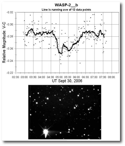
Last night (Fri/Sat) I tried for WASP2 and got some data that looks promising. The data is very noisy and I would not feel comfortable about presenting it without some other confirming (hopefully someone else got data) observations.

I have attached a .jpg image of the data chart. The data is really forced to get any kind of “curve”. The solid line represents a running average over 16.25 minutes, 13 data points.

The individual images are 65sec at an interval of 75 sec. The scope is 200mm @ f/8 with a Cookbook 245 CCD, no filters.

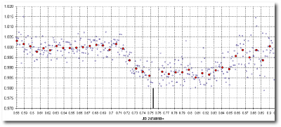
Here’s his lightcurve:

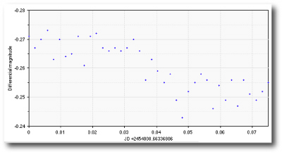
Today, Geir Klingenberg from Norway checked in with a confirmation of Garlitz’s result (which he obtained remotely from a telescope in New Mexico:

Hi Joe,

I observed the ingress of this WASP-2 transit, see here.

Seems to fit your data nicely.

I used a robotic telescope at GRAS: 0.3m SCT @ f/11.9 and a FLI IMG1024.

Way to go, guys!

The golden ratio

It was gratifying to watch the first systemic challenge unfold.

After a week of accepting fits, we tallied the entries and determined that Chris Thiessen had obtained to the lowest submitted chi-square. Way to go Chris! Eugenio then added the “challenge001” data set to the systemic backend, so that users can continue to improve and submit fits.

So what was the underlying synthetic planetary configuration that generated the data set?

Both Eugenio and I have had a long-running interest in the GJ 876, a 15-light year distant red dwarf star that is now known to harbor at least three planets. The two outer worlds in the system, which were discovered in 1998 and 2001, are in 2:1 resonance, and form the classic example of a configuration that demands a self-consistent (as opposed to Keplerian) model. Last year, Eugenio led the discovery and characterization of a third planet in the system, which has a mass only 7.5 times that of Earth, and orbits the star every 1.94 days. (Here’s a link to the NSF press release for Rivera et al. 2005.)

We’ve been looking into the possibility of detecting another planet in the system, and in order to do so, we’ve been studying synthetic data sets that contain the three known planets, as well as a fourth, potentially habitable planet in a potentially habitable orbit. The following table gives the parameters of our hoped-for system (which, like the real system, has its invariable plane inclined by 40 degrees with respect to the line of sight.)

(JD 2452490)
Parameter Planet 1 Planet 2 Planet 3 Planet 4
Period (days) 1.937747 7.106642 30.45123 60.83227
Mass (M_Jup) 0.025101 0.016193 0.791650 2.531229
Mean Anomaly (deg) 308.84845 169.44032 312.3738 159.1070
eccentricity 0.000000 0.000000 0.262795 0.033979
omega (deg) 0.000000 0.000000 195.8324 191.9573

The first 155 points in the challenge data set used the actual observing times given in Rivera et al 2005. The remaining 32 points were generated using the version of Eugenio’s Keck_TAC program that we use to produce the systemic synthetic data sets. We then subtracted off the the first epoch time from all 187 observing times and multiplied each of the resulting times by the golden section, 1.618033989. This gives a system that has the dynamical characteritics of the real GJ 876 system, but with orbital periods that are all 1.618 times longer.

After setting up the uploads page on the backend, Eugenio uploaded the best fit that he was able to obtain, which had a chi-square of 3.13. A lot of computation went in to getting this fit, which took several days on a fast desktop machine.

Amazingly, the next day, user Roseundy submitted an even better fit,

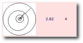
which brought the chi-square down to 2.82, with the following comment:

Arrrggghh!!!!!!!! I had this fit on Sep 13, but I thought the ChiSq was too high to bother to submit. Lesson learned.

Eugenio and I were quite excited. Systemic users have clearly gotten at least as good at fitting with the console as we are, and we have been thinking carefully about the problem for quite a while. In the comments section on Roseundy’s fit, Eugenio wrote:

Hi Roseundy, That is awesome work!! All the challenge systems will be based on some known model, possibly a random draw, some noise, and possibly other effects. The random draw and the noise complicate the situation for the modeler (me), so that knowledge of the model will not always result in the best fit. Actually, your result is a major success for the idea behind the systemic collaboration — distributing the process of fitting radial velocity data sets. Because I really don’t know precisely how the random draw and the noise affected the model, it may still be possible to get even lower chisq values. I encourage everyone to continue fitting this system (as well as others). It does require patience and perserverence.

Chris Thiessen wrote:

Roseundy, I’m very impressed. The two major planets have such different Keplerian and integrated fits that I was never able to get them to work well together. How did you get the two planet solution? I’m not sure I would have let the 48 day planet develop that much eccentricity if I’d seen a trend. Maybe I missed out that way. Great work!

Whereupon Roseundy revealed the secrets of his fitting method:

Once I saw how close the planets were, I realized I needed to work with integration turn on. This, of course, slowed things down painfully. To make progress, I cut down the dataset (the middle third of the velocity data) and played with that until I got a good (chi^2 of 7 or so) fit. I backed that out to the full data set (very painful) and then added additional planets based on the residuals. I polished until I got the fit you see. I’m sure it can be improved, but I lost patience with it. I would like to see three improvements to the console to make this easier in the future: 1. be able to subset the data 2. be able to select which planets are to be integrated together, using Keplerian calculations for the rest. this would help with systems where only a few planets substantially interact with each other 3. (my vote for the most important) a natively compiled console. java byte code may be portable, but I don’t it’s very optimized. Having optimized binaries (x86 on Linux preferably) would be a win, I think.

We agree. After the next release of the console, I think it would be a good idea to migrate to a strategy where the systemic community of users can work on the console code open-source style. This is clearly another area where a distributed attack will get important and interesting results.

In any event, thanks to everyone who has been reading the oklo blog and collaborating in the backend. We’ve had over 6,000 unique visitors so far this month, and the project is really starting to show promise.

The Second Challenge System

Image Source.

The second systemic challenge radial velocity dataset is now included on the downloadable systemic console. This system is dynamically quite interesting, and also possibly quite scientifically relevant. It’s non-trivial to fit, and integration is required in order to produce a viable model. The computational demands, while modestly high, are nowhere near what was required to crack the first challenge system.

Send your entries to me at the e-mail address given on the web page listed in the Sky and Telescope article. (Same procedure as previously).

Note that the downloadable console currently does not include the massive synthetic data sets for Alpha Centauri. These data were causing download times to become excruciatingly slow. Later this week, I’ll write a post which explains how the Alpha Centauri data sets can be accessed, and which also explains how the console can be updated without downloading an entire new package. (For the time being, though, you are best off just downloading a fresh copy.)

The first challenge system is now included in the systemic backend, with Eugenio’s solution posted. (Chris Thiessen was the winner of the contest). Feel free to submit additional fits, and in the next post or two, I’ll give a discussion of what’s going on dynamically in that system.

And the Winner is…

I’ve evaluated the fits submitted for the first Systemic Challenge radial velocity data set, and the winner is Chris Thiessen.

In addition to being dynamically interesting, the configuration proved to be very tough to crack. The challenge 001 system is one where a Keplerian model can reach a low chi-square, which then skyrockets when the planets are actually integrated through their orbits.

I’m travelling today, without full access to the Internet. In the next day or so, once I get back to the office, I’ll put up a more detailed post which looks at what’s really going on in the first challenge system. We’ll also release the second challenge data set (which is equally interesting, but a lot more tractable).

last call

If you’ve been working on the first systemic challenge system, please submit your fit as an ascii file to the e-mail address listed on the web-page given in the Sky and Telescope article. At 00:00 UT Sept. 14th (JD 2453992.5) I’ll close the submissions and see who wins the Star Atlas.

Don’t hesitate to submit if your chi-square is still far from 1.00. Our first challenge system turned out to be a bit harder than we anticipated. Next week’s system will be equally interesting from a dynamical point of view, but will be a lot easier on the ol’ CPU.

HD 208487

Image Source.

An relevant paper showed up on the astro-ph preprint server this morning, “A Bayesian Kepler Periodogram Detects a Second Planet in HD 208487” by P. Ç. Gregory of the University of British Columbia.

Gregory employs a technique known as the parallel tempering Markov Chain Monte Carlo algorithm to argue that the HD 208487 data set contains two planets. The first planet (which was previously announced by Tinney et al. 2005, and confirmed by Butler et al. 2006) has a period of 130 days and a minimum mass 37% that of Jupiter. The second planet in Gregory’s model lies out at a period of 908 days, and has 46% of Jupiter’s mass.

Interestingly, the console does not recover Gregory’s parameters precisely, but it does find a fit that’s extremely similar. (I just uploaded the fit to the systemic back-end.) The radial velocity reflex curve looks like this:


wheras the planetary configuration (at the moment when the first radial velocity data point was obtained on Aug. 8th, 1998) looks like this:

It’s interesting to look at the fits for the latest HD 208487 dataset that have been submitted by participants in the systemic collaboration. At the moment, there are six different fits:

On September 4th, mikevald submitted a 2-planet fit that is a close analog of the one published by Gregory. In the last several days, dstew and andy have also turned in fits that have essentially the same configuration as obtained by Gregory. That’s definitely cool.

In addition to the five fits that look like the Gregory configuration, with the outer planet at a period of P~1000 days, there’s also a completely different take on the system that was submitted this morning by Olweg. In the Olweg fit, the second planet lies interior to the known planet, and has a period of only 29 days. The chi-square is less than one, indicating a slight degree of overfitting. When overfitting occurs, it can easily be remedied by a slight random perturbation of the parameters. It’s very interesting that this fit was completely missed by the Bayesian Kepler Periodogram, so I thought I would have a closer look at Olweg’s model system.

The Olweg radial velocity curve is radically different from the Gregory fit:

The 28.68 day inner planet has a mass of 0.16 Jupiter masses (about 50 Earth masses) and travels on an orbit of modest (e=0.18) eccentricity. There’s a fair amount of planet-planet interaction in this system over the time scale of the radial velocity observations. By the time the fit reaches the end of the data set, there’s a noticeable difference between the keplerian model fit and a self consistent (integrated) model fit:

The system is stable, however, when I did a short test integration of 100,000 years. The secular interaction between the two planets causes the two orbits to execute a complicated dance over a timescale of several thousand years, with the periastron angle of the inner planet orbit mostly librating around an anti-aligned configuration.

As I’ve remarked in an earlier post, we’re currently in the progress of upgrading the downloadable console so that it will be capable of computing estimates of the uncertainties in the orbital elements of a fit. A good way to generate uncertainties in this context is to use the so-called bootstrap method. In the bootstrap, one re-draws the original radial velocity data set with replacement, thus producing alternate realizations of the data in which a fraction of the points appear more than once, and in which a fraction do not appear at all. One then fits to these new datasets, thereby building up distributions for each orbital element. (For more detail, see this paper, which describes in detail how this procedure was applied to the radial velocity data set for HD 209458.) When I run a self-consistent bootstrap analysis based on the Olweg fit, I get the following mean values and standard deviations for the parameters:

This fit is thus quite well constrained, and is a completely viable competing model for describing the hd208487 planetary system. I think the situation here really underscores the value of the systemic collaboration. Many radial velocity data-sets can be fitted by completely different models that offer equally robust fits to the data, while simultaneously maintaining small uncertainties on their bootstrap-estimated parameters.

So how do we know which HD 208487 system (if either) is correct? I’m hoping that the Monte Carlo simulation that will make up phase II of the systemic project will give a great deal of insight into when a particular orbital model can be deemed secure.

desiderata

strands of wheat

Image Source.

It’s good to see that users are still streaming into the systemic collaboration, and activity on the back-end is staying strong. The catalog of submitted radial velocity fits is now approaching 1,000 entries, and nearly every data-set has at least one fit. We need more users, though. Both Stefano and Eugenio have been working very hard behind the scenes to engineer improved usability for the site. There are a lot of items that are still on our plate, but progress is definitely being made.

We can now internally query the database of submitted fits to statistically characterize the planetary models that are being submitted. Once this functionality is fully tested, it’ll be made available to all users on the site. For example, here’s a plot of eccentricity vs. period for all of the fits submitted with 0.8 < chi-square < 2.0: aggregated P-e diagram

It’s interesting to compare this with the plot that one can produce at exoplanet.eu based on the static catalog of published planets:

One immediately notices that the diagram produced from the back-end data is populated in the upper left hand corner, whereas this region in the published catalog is completely cleared out. Note that planets in this region are known from theoretical arguments to be tidally circularized… (tune in soon for more on that issue).

One final note. The downloadable console is now much lighter. The large filesize of the previous version was due to the very extensive synthetic data sets for alpha Centauri. If you want the alpha Centauri velocities, the fully loaded console that contains the alpha Centauri data is here. Within a day or so, we’ll be updating the downloads page to reflect this change and to give more guidance for International Windows users.

New Texas V’s

Image Source.

Data data data. Robert Wittenmyer and his colleagues at the University of Texas have just posted a paper on astro-ph that contains a slew of new radial velocities for several famous planet-bearing stars, including 47 UMa, 14 Her, and 16 Cyg B. The velocities are all tabulated in the paper, so we’ll have them up on the systemic backend very shortly. [I’ll post a comment to this post when they’re up on the site. If you’re totally gung ho to get them right away, you can extract them from the posted latex file at astro-ph, and then add them manually to systemic’s datafiles directory.]

We always try to add new radial velocity data sets as soon as they become publicly available, and lately, these updates have been occurring roughly once per week. For the time being, the simplest way to get your fresh V’s is to rename your old systemic directory, and then download a new console. When the new console and catalog data are downloaded and unzipped, you can copy any previous fits and soundfiles that you’ve created into the new fits and soundClips directories.

The data in the Wittenmyer paper come from both the Harlan J. Smith 2.7-meter telescope and the Hobbey-Eberly 9.2-meter telescope. The cadence of the Smith telescope observations typifies the usual pattern of radial velocity survey data. The individual points are spaced essentially randomly in time, with many days separating each point. The Hobbey-Ebery data, on the other hand, are quite different. These data are much more densely sampled, and many nights contain several velocities in succession. In many stretches, the star is observed every few nights. This pattern results from queue-scheduling, which enables very intensive monitoring of systems that are of particular interest. I think queue scheduling is the wave of the future, and in the systemic simulation, we’ll have many synthetic data sets whose cadences correspond to the queue-scheduled approach.

The most prominent planet orbiting 14 Her has been known since the late 1990s. This world, known as 14 Her “b”, has a minimum mass about 4.6 times that of Jupiter, and a period of ~1770 days. If it were in our solar system, it would orbit in the asteroid belt. The parent star 14 Her is about 90% as massive as the Sun, and is more than twice as metal-rich. Given the planet-metallicity connection, it’s absolutely no surprise that 14 Her has a heavy-duty planetary system. I bet that 14 Her “b” has a very interesting system of satellites.

It’s pretty clear from the one planet fit that 14 Her “b” is not the only planet in the system, and over the weekend, several systemic users have submitted interesting fits to the data that reduce the chi-square by adding a second planet. For example, on August 30, user mikevald uploaded a two-planet fit in which the second planet, 14 Her “c”, has a period of 6159 days and an eccentricity e=0.52. This model currently fields the lowest chi-square statistic of any of the submitted 14 Her fits. The orbits in this best-fit system are crossing, however, indicating that the model may not be dynamically stable over the long run. On September 5th, allanfloering submitted a fit with nearly as good a chi-square, in which the outer planet has a 14,669 day period and an eccentricity e=0.09. Allanfloering’s world, if it exists, lies 11.77 AU from 14 Her, out at a Saturn-like distance.

Wittenmyer et al. show that the addition of their new 14 Her data suggests that 14 Her “c” has a period of order 6900 days, albeit with a low eccentricity. In their models, “c” and “b” may be participating in 4:1 resonance. A quick fit on the console with the Wittenmyer et al data included gives a radial velocity curve that looks like this:

corresponding to a planetary configuration that has an outer planet with a modest eccentricity e=0.20.

As soon as the data go up on the site, feel free to try working up improvements. It will be interesting to see how many fits to the full 3-telescope data set are participating in 4:1 resonance.

Web 2.0

fenceposts at ucsc

Hey ya’ll, there’s a whole lotta fittin’ goin on out there in the back 40.

Seriously, though. We’re really seeing a great response from users who are contributing their efforts. Nearly 200 people have registered on the back-end during the past few days, and over 750 different radial velocity fits have been uploaded. Hopefully we’ll see that work continue to flow in, and everyone has been showing admirable patience as we smooth out the inevitable rough spots which began to show up as soon as we had a surge of real users on the site.

If you’re arriving by way of the Sky and Telescope article, you’ll notice that the full universe of 100,000 synthetic stars is not yet listed on the systemic backend. During September, we’re still carrying out the first phase of our planned research effort, which consists of accumulating a wide variety of fits to the full collection of actual, published radial velocity data sets. Very soon, we will have accumulated enough fits to be able to present a dynamic, interactive catalog of candidate planets. A query-based dynamically generated planetary catalog will allow a variety of very interesting questions to be answered. For instance, by how much can one deflate the famous eccentricity-period diagram, while still demanding a prespecified goodness-of-fit for all of the candidate planets?

generated at exoplanet.eu

At the moment, such questions are hard to answer, because (other than here at oklo) there is no consolidated repository of radial velocity data and associated self-consistent fits.

In order to make dynamically generated planet catalogs scientifically useful, we’re going to have to provide several more tools to the users. As I mentioned yesterday, the console will soon be multi-threaded, which will make it easier to use for high-performance work. In the interim, however, you can have the console print a stream of diagnostic messages by launching it from the command line. For example, on linux or OSX architectures, open a terminal (shell), cd to the systemic directory, and type java -jar systemic.jar at the prompt . The diagnostics provide a running update of the progress of the console as it produces fits to the data set.

We’ll also soon be providing a long-term integration window that will allow users to verify that their model systems are dynamically stable. It’s alarmingly easy to find multiple-planet fits to radial velocity data sets that have low values for the reduced chi-square statistic, but in which the planets experience dynamical disasters (collisions, ejections, close encounters, etc.) on a time scale that is short in comparison to the known age of the parent star. Indeed, most of the candidate stars in the back-end catalog are more than 2 billion years old. Young stars tend to be rapidly rotating, which broadens their absorption lines and makes radial velocity measurements less accurate. Rapidly rotating stars also tend to have elevated levels of magnetically driven chromospheric activity, which adds additional noise to the velocity estimates.

And finally, the console needs to provide error estimates on the orbital parameters that it generates. This is best done using the so-called bootstrap method, which we’ll discuss in an upcoming post.

Systemic Challenge — data set #1

Image Source.

We’re continuing to see a strong influx of new users and activity on the systemic backend. Thanks to everyone who’s taking part! If you’re a first-time visitor to the Systemic Project website, please read the weblog entries that follow this post. They contain the information you need to start participating, and they give a recent day-by-day overview of the project developments.

Now that we’ve got an active user-base for the systemic console, we’re pleased to release the first Systemic Challenge synthetic radial velocity data set. This data set corresponds to a realistic simulated planetary system that is both scientifically interesting and non-trivial to fit.

Sky and Telescope is sponsoring the world’s first radial velocity fitting contest in connection with our challenge system. The person who submits the self-consistent (integrated) fit to the data having a chi-square value closest to one will receive a paperback edition of the Millennium Star Atlas (a $149.95 value).

Continue reading

consolidation

Image Source.

Wow! The American Scientist and Sky and Telescope articles are clearly getting the word out. We’ve been seeing a significant increase in traffic on the oklo.org site, both in terms of visits (yellow bars) and bandwidth and page views (green and blue bars). The bandwidth increase is especially gratifying. It reflects the fact that many users are registering on the back-end, downloading the console, and submitting fits. As I write this, new and interesting fits for a variety of different radial velocity data sets are rolling in to the star catalog. Our goal of fostering original, public-participation exoplanet research is starting to be realized, and I want to thank everyone who’s lending a hand.

Late August stats.

If you’re a first-time visitor to the Systemic Project website, please read the blog entries that were posted prior to this entry. They contain the information you need to start participating, and they give an overview of the current project status. If you are a return visitor, please have a look at the updated back-end. Stefano has made a number of code and design improvements that streamline the workflow and make the site easier to navigate.

On to some planet issues. The Mu Ara (HD 169061) system, which contains four known planets, is shaping up to have significant implications for the systemic project. Intense interest in the system has been spurred by a recent paper from the Swiss group (Pepe et al. 2006) that presents a self-consistent 4-planet model. Pepe et al.’s orbital fit (given in their Table 1) provides an excellent match to the radial velocity data sets, but when they carried out a long-term integration of the system, they found that the gravitational interactions between the planets lead to catastrophe after 76 million years. The parent star Mu Arae has an estimated age of 6.4 billion years, so clearly we don’t yet have a full understanding of what’s going on with this system.

The discord within the Pepe et al. model is provided by the two middle planets, one of which has a 310 day orbit, and the other which orbits in 643 days. The planets are on the edge of the 2:1 mean motion resonance, with the practical consequence that they experience a strongly chaotic orbital evolution. The orbits change eccentricity and orientation on a timescale of only decades:

I’ve made a movie that tracks the evolution of the orbits over 528 years. Here are links to a .mov version (288 kB) and an .mp4 version (1.5 MB). It’s clear from the movie that the interaction is both complicated and unpredictable. The planets display no catastrophic excursions on the 500 year timescale of the movie, but eventually, they experience orbit crossings leading to a likely ejection of the inner 0.5 Jupiter mass planet.

The Mu Ara dataset HD169061_B06P06CH on the console back-end combines both the Pepe et al. data as well as the most recent data from Butler et al. 2006. I’m hoping that someone can get a stable, self-consistent, low chi-square fit to this combined data set. Such a fit would give the best available view of what’s going on with the system, and would underscore the scientific relevance of the systemic project.

more updates

We’ve been seeing a nice increase on traffic here at oklo.org as the Sky and Telescope and American Scientist articles show up in mailboxes and on newstands. If you’re new to the site, welcome aboard, and please read the last several posts. They give a brief overview of the Systemic Project, and tell you what you need to start fitting systems.

As you may have noticed, we’re hard at work improving the usability of the site. Stefano, in particular, has done an amazing amount of work on the back-end over the past several days. It really is taking shape as a genuine research environment, and we absolutely are urging you to try it out while we’re putting the definitive users manual together. You can’t break anything, and if you post questions, we’ll make sure they get answered on a timely basis.

A few news items:

(1) There are two separate channels for registration on systemic. The first, accessed through the “login” tab on the site header above, is part of the WordPress package that runs the oklo blog. Registration on the blog allows you to comment on the oklo.org posts. The second, accessed through the “backend” tab on the site header, gives you access to the collaborative php-based environment that constitutes the systemic backend. You can register for either or both, and you don’t need to give your real name or any real-world identifying information other than an e-mail address.

(2) We’ve been working to design the first systemic challenge radial velocity data set, which will be released on Monday September 4th. The user who finds the fit with a reduced chi-square closest to unity will win a $149 Sky Atlas from Sky and Telescope. Both professional and amateur planet hunters are encouraged to participate, but given the groundswell of activity that we’re seeing on the systemic back-end, and given the console’s ability to carry out self-consistent fits, the smart money is on an amateur winner.

Updated back end

Image Source.

Stefano (while in the midst of writing his astrophysics thesis in Bologna!) has somehow found the time to implement a whole slew of very cool improvements to the Systemic back end. New aspects include a search function, a personal “fits” library, and a variety of interactive features designed to aid collaboration and make the user experience more rewarding.

We’re working on a full user manual for both the downloadable console and the back end, but in the meantime, we’re really urging users to (1) download the console, (2) create a free account on the back end, (3) work through the systemic console tutorials one, two, and three, (4) upload fits, and (5) start collaborating. There are a number of real systems in the star catalog which can be profitably characterized and improved. I’m also very interested to see what people come up with for the datasets systemic001 and systemic002.

Do give it a try, and please give us feedback, either in the comments section on the back-end, or in the comments section for this post.

Two tips: (1) For Mac-users, Firefox provides a better interface to the back-end than does Safari. (2) At the moment, the user-interface looks better if you resize to a wider browser window.

The mu Arae four

flowerstalk

Image Source.

With the verdict in on Pluto, we here at oklo.org will have to revert to sober, scientifically rigorous posts on extrasolar planetary systems to keep our readership and ad rates up. And as soon as I can figure out how to make WordPress launch those “swing for the fences” pop-ups from our site, we’ll be increasing our revenue stream even more.

American Scientist has just published my article on planet formation and extrasolar planets in their September/October issue. The article wraps up with a description of the systemic console, and the systemic collaborative research project. If you’re an American Scientist reader visiting oklo.org for the first time, welcome aboard!

Several posts back, I put up a brief description of the immediate goals of the Systemic collaboration:

The Systemic collaboration is proceeding in three steps. In the first step, which is ongoing, we’ve been gathering all of the radial velocity data that have been published for known planet-bearing stars. These data sets are included in the downloadable systemic console, and the systemic back-end allows participants to upload their own planetary fits to this data. We want to use the data to create a uniform catalog of known planetary systems.

In the second and third phases of the systemic project, we’ll be studying synthetic data sets that have been produced using our own algorithms. “Systemic Jr.” will launch at the beginning of September, and will contain 100 synthetic data sets, four of which will be special challenge systems. The Systemic Challenge, sponsored by Sky and Telescope will be explained in more detail, and will be available at a link on their website. The challenge systems will be released on September 3, 10, 17, and 24, along with a specific set of contest rules. The first person to crack each of these systems will recieve a paperback edition of the Millennium Star Atlas (a $149.95 value). In order to prepare for the contests, go ahead and download a copy of the systemic console, and work through tutorials one, two, and three. A full technical manual for the console is in the works, and will be ready for download quite soon.

Later this Fall, when Systemic Jr. wraps up, we’ll launch the full Systemic simulation. A lot more on this will be posted in the weeks ahead. Our overall goal is to obtain an improved statistical characterization of the galactic planetary census.

The most interesting serious-planet news from the past week has been the paper by the Geneva Extrasolar Planet Search Team that releases an updated radial velocity data set for the nearby solar-type star Mu Arae (also known as HD 160691). As discussed in this post, the console can be used to quickly uncover and characterize the orbits of the four planets that have been announced for the system.

The mu Arae system is remarkable because the two middle planets (with periods P~300 days, planet “d”, and P~640 days, planet “b”) experience strong mutual gravitational interactions during the 5-year time period that the system has been observed. The presence of strong interactions indicates that a model for the system built from independant Keplerian orbits cannot provide a fully realistic fit to the system. In order to build a fully self-consistent fit, one must find an N-body model. The systemic console has this ability, which is enabled whenever the “integrate” box is checked.

N-body integrations are much more time-consuming to compute than simple evaluations of Keplerian fitting functions. The performance of the console thus slows down considerably when integration is enabled. (Note also, that this post now becomes a bit technical. If it sounds like gibberish, you can either skim the next few paragraphs, or, better yet, work through the tutorials on the use of the console.)

Continue reading

Roll your own.

succulent

Image Source.

The October 2006 issue of Sky and Telescope is just hitting the stands. It contains a feature article — Virtual Planet Sleuths — on the usage of the console and the Systemic collaborative project. If you’ve read the Sky and Telescope article, and are a first-time visitor to oklo.org, welcome aboard!

The Systemic collaboration is proceeding in three steps. In the first step, which is ongoing, we’ve been gathering all of the radial velocity data that have been published for known planet-bearing stars. These data sets are included in the downloadable systemic console, and the systemic back-end allows participants to upload their own planetary fits to this data. We want to use the data to create a uniform catalog of known planetary systems.

In the second and third phases of the systemic project, we’ll be studying synthetic data sets that have been produced using our own algorithms. “Systemic Jr.” will launch at the beginning of September, and will contain 100 synthetic data sets, four of which will be special challenge systems. The Systemic Challenge, sponsored by Sky and Telescope will be explained in more detail, and will be available at a link on their website. The challenge systems will be released on September 3, 10, 17, and 24, along with a specific set of contest rules. The first person to crack each of these systems will recieve a paperback edition of the Millennium Star Atlas (a $149.95 value).

Later this Fall, when Systemic Jr. wraps up, we’ll launch the full Systemic simulation. A lot more on this will be posted in the weeks ahead. Our overall goal is to obtain an improved statistical characterization of the galactic planetary census.

In the Sky and Telescope article, I made a rather bold claim that by using the console, it’s possible to find an as-yet unannounced planet around more than a dozen different stars. The 55 Cancri data set, for example, is an excellent place for aspiring planet hunters to try their hand.

The feasibility of detecting planets in the published data sets was illustrated dramatically over the past week. On August 14th, Krzysztof Gozdziewski, Andrzej Maciejewski, and Cezary Migaszewski posted a preprint on astro-ph which describes their detection of a fourth — then unknown and then unconfirmed — planet orbiting HD 160691 (also known as mu Ara). They detected the planet using their own software, which has a similar set of capabilities to the systemic console, and they used the dataset provided by the recent Butler et al. 2006 catalog paper. They found an orbital period of P~307 days for the planet, a nearly circular orbit, and a mass of 0.5 Jupiter Masses.

Today, on astro-ph, the Geneva Radial Velocity Search team published a paper with an updated set of radial velocities of HD 160691 which were obtained with the HARPS instrument at La Silla. In the abstract of their paper, they write: “We present the discovery of mu Ara d, a new planet on an almost circular 310-days period and with a mass of 0.52 Jupiter Masses”.

So there you go, folks! The planets are in the data sets. You just need to download the console, fire it up, get a good fit, and submit it to the Systemic back-end.

[Note: It’s not clear what (if any) “credit” Gozdziewski et al. will get for their discovery. I don’t want to proffer an opinion on who should get credit in a case like this, mainly because I really don’t care. The Systemic backend includes a public-record chronological list of submitted fits for each radial velocity data set. If you turn up a planetary configuration that later gets confirmed by one of the radial velocity teams, you’ll get the personal satisfaction of knowing you knew about the planet first. What you almost certainly won’t get, however, is official credit for the discovery, or the right to name the planet, etc., etc.

For the synthetic planets in phases 2 and 3 of the Systemic collaboration, however, the discoverers will receive official credit, and they will have the right to name the planets if they choose to do so.]

Synthesis

The Dragon at the Kurama Shrine

Potentially the most interesting feature on the downloadable systemic console is the “sonify button”, which integrates the model planetary system specified by the state of the console sliders and produces a .wav format CD-quality audio file of the resulting radial velocity waveform. Not interested in planets? The console is a stand-alone non-linear digital synthesizer. It’s capable of producing strange, remarkable, musically useful sounds. They merely need to be located within the uncountable infinity of solutions to the gravitational N-body problem.

First, use the console to build an interesting multi-planet system (for this purpose, there’s no need to try to fit whatever data is in the window.) Then click the sonify button. This brings up a dialogue window which enables the user to make several specifications for the sound file that is produced.

console sonify dialogue box

The most important user-specified parameter is the frequency onto which the orbital period of the shortest-period planet on the console is mapped. If, for example, the innermost planet has a period of 365.25 days, then a 440 Hz map will play 440 years worth of evolution in one second. (440 Hz corresponds to the A below middle C.) Mapping the radial velocity curve onto a high-frequency note extends the total number of orbits that go into the sample, and thus increases the integration time required to produce the sample. You can also specify the length of the sample, and you can exert simple control over the attack and decay rate of the envelope for the overall waveform.

Once you’ve produced the soundfile, it appears in the “soundClips” subdirectory within the systemic parent directory. Both of these directories are automatically created when you download and expand the console — see the instruction set for the downloadable console for more details. With a Macintosh, you get the best results if you play the sample right from the folder. i-Tunes seems to want to convert the samples to .mp3 format in a manner that introduces audible noise, and we’re not yet sure how to resolve this issue.

To the extent that planets orbit independently of one another, the console behaves like a simple additive synthesizer, in which the individual Kepler waveforms add to form a composite sound. Much more interesting, is the situation when planets experience significant gravitational interaction, leading, for example, to resonance and to nonlinear instability (here are examples, 1, 2, from the resources page of both types of waveforms). Close encounters provide discontinuities between individual blocks of sound that resemble the results of granular synthesis.

The strongest 2-planet mean-motion resonances occur when the pair of planets share a common period and engage in a one-to-one resonant motion. There are a variety of different one-to-one resonances, including binary planet orbits (e.g. Earth and Moon), trojan configurations, and generalizations of retrograde satellite orbits. In this last catefgory, one can have two planets with the same semi-major axis, but with different eccentricities. If one starts the planets in the following configuration, then the motion is dynamically stable, and evolves in a complicated way over time.

evolution of eccentric 1:1 resonance

The motion leads to an interesting audio wave-form, in which you can hear the system cycling between configurations in which both planets are modestly eccentric and configurations in which one orbit is nearly circular while the other one is highly eccentric. As a specific example, set the console to the following configuration: P1=P2=10 days, M1=M2=0.3 Mjup, MA1=180., MA2=190., e1=0.9, e2=0.1, long1=0.0, long2=0.0. If you increase MA2 to about 225 degrees while keeping the other parameters fixed, you’ll hear the system go unstable.

Evolving, high-eccentricity orbits tend to have an insect-like quality, which brings to mind the 1986 album, The Insect Musicians, by Greame Revell (formerly of SPK). From the album jacket:

For the two years 1984-85, Graeme Revell travelled from Australia to Europe, to Africa, Indonesia and North America recording and negotiating copyrights of insect sound recordings. It took another full year sampling and metamorphosing some fourty sounds thus gathered using the Fairlight Computer Musical Instrument, to produce this record. The only sounds used are those of insects, altered digitally and combined into a unique orchestra of instruments, an orchestra of strange and delicate timbres, music of natural rhythm and texture.

extraterrestrial

thistle against a white background

Image Source

We’re working hard to keep the systemic project moving forward.

Eugenio, as of July 14th, has compiled and documented all of the published radial velocity data sets, and has been designing and developing the “KeckTAC” code, which will be a workhorse for systemic’s next phase. The published datasets are all available on the systemic systems catalog. Aaron has stripped the console down to its component parts, and he’s rebuilding it with new features, faster algorithms and a sleekly expandable architecture. Stefano has been tweaking the systemic backend [sign up and get fittin’, y’all -ed.], and will be arriving at UCSC in the Fall to do his Ph.D. research. We’re hoping that part of his thesis will be a statistical analysis of the final results of the 100,000 star systemic simulation.

When I was in graduate school, I spent a lot of time doing research on brown dwarfs (objects between 13 and 75 Jupiter masses that lie in the mass range between giant planets and red dwarf stars). At that time, circa 1992, no bona-fide brown dwarfs had actually been found, but the prospects for detecting them seemed reasonably good. My friend Todd Henry, who was a graduate student at the University of Arizona, and who was hunting for brown dwarfs using the speckle method, told me something that stuck in my mind.

“Face it, Greg,” he said, “the reason you’re interested in brown dwarfs is not because you’re interested in Brown Dwarfs — the reason you’re interested in brown dwarfs is because you’re really interested in planets, and brown dwarfs are just one stop away on the line.”

He was right.

A similar logic might apply today, “The reason I’m interested in giant planets is not because I’m really interested in Giant Planets — the reason I’m interested in giant planets is because I’m really interested in habitable terrestrial planets, and giant planets are one stop away on the line.”

Good Librations

Janus and Epimetheus

Janus and Epimetheus Source: JPL

Last week, I wrote a post about the negative heat capacity of self-gravitating systems. I never cease to find it remarkable that if you drain energy out of a system that is held together by its own gravity (such as a giant planet, or a cluster of stars), then that system gets hotter. There really is such a thing as a free lunch, brought to you courtesy of the attractive gravitational force.

A collection of bodies orbiting a larger body is a self-gravitating system, and therefore will also display a negative heat capacity. We illustrated this with the idea of a satellite running through a cloud of dust. Friction between the satellite and the dust heats both bodies up, and they radiate energy away to space. The satellite simultaneously spirals into an orbit with higher velocity, and hence a higher kinetic energy, or temperature.

A family of orbital trajectories known as horseshoe orbits present a riff on this basic principle. A horseshoe orbit occurs when two bodies, with slightly different orbital periods, start off in near-circular orbits on opposite sides of a large central mass. The body with the shorter orbital period eventually attempts to overtake the body with the longer orbital period.

As the short-period body catches up with the long-period body, an attractive gravitational force is exerted between the pair. This force pulls the short-period body forward, and pulls the long-period body back. That is, the gravitational interaction leads to an exchange which drains orbital energy from the long-period (leading) body, and gives energy to the short-period (trailing) body. This exchange causes the bodies to swap orbital periods. The long-period body gets a shorter period, and the short-period body gets a longer period. In a frame that rotates with the average orbital velocity of the pair, the two bodies eventually come in to contact again on the opposite side of the star, and the process is repeated. Again and again in an mindlessly delicate cycle.

dynamics of the horseshoe orbit

The orbital trajectory in the above figure is lifted and adapted from a paper in the Astronomical Journal that I wrote with John Chambers. In that paper, we studied a number of weird co-orbital planetary configurations, and speculated that they might eventually be observed using the radial velocity method. If you can’t fit a particular data set with the console, the horseshoe configuration is always a good thing to check.

In our own solar system, there are two small Saturnian moons, Janus and Epimetheus, which are caught in a horseshoe-like orbit. The splash picture for today’s post shows a Cassini photograph of these moons taken near the time during which they exchange periods.

One of the most useful features of systemic console is its ability to sonify radial velocity waveforms. The soundfiles are produced by making a full integration of the equations of motion, hence all of the nonlinear gravitational interactions between the bodies are incorporated into the sound. When the console is used as a nonlinear digital synthesizer, the horseshoe orbits provide a method for producing amplitude modulation of a tone. To see how this works, launch the downloadable console, and set up the following system (just ignore the radial velocity data, since we’re not interested in fitting, but rather just in waveform generation):

console for a horseshoe orbit

That is, set up two 0.2 Jupiter mass planets with mean anomalies of 0 and 180 degrees. Make the period of one planet 10.1 days, and the other 10.0 days. For simplicity, keep the eccentricities at zero. Clicking the integration box shows the resulting radial velocity waveform. When the planets are on opposite sides of the star, their radial velocity influences on the star cancel. When they are on the same side of the star, their radial velocity influences are additive. This gives an overall modulation envelope on top of the fundamental ~10.05 day period. Use the sonify button to create a 220 hz tone out of this system:

sonifier

Here’s a link to the resulting .wav file. The amplitude modulation (or tremolo) can clearly be heard.

Try building some more complex sounds by nesting horseshoe orbits, and using unequal masses. If you get something cool, e-mail me at laughlin ucolick edu.

cleanse, fold, and manipulate

Thanks to everyone who has created an account on the systemic backend, downloaded the console, and submitted fits to the HD 69830 data sets. It’s gratifying to see the collaborative effort coming together. We’re starting to get a better understanding of which aspects of the HD 69830 data set seem secure, and which aspects are uncertain.

That outer planet seems to me to be leaning toward the latter category.

For example, I just had a look at data set #17 for HD 69830. Guided first by the console’s periodogram and then by the console’s residuals periodogram, I worked up a two planet fit to the data. I kept the orbits of the resulting 8.66 and 31.7 day planets circular. In the absence of strong planet-planet gravitational interactions or resonant disk migration, I don’t see a clear rationale for assigning non-circular orbits unless the data really demands it.

The residuals periodogram of the 2-planet fit above has peaks near 200 and 400 days. The 200 day peak is a little higher, and indeed, corresponds to the outermost planet announced in the Nature paper published last week.

Use the folding window to look at the case for the 200 day planet. Try updating the period in tiny increments, and watch the data congeal into a relatively sinusoidal pattern. The third planet in the published fit is based on this configuration:

The 400 day data also looks good (although the power is not quite as high). Notice, too, that the phase coverage near 400 days is not as good. This is due both to the limited time baseline of the whole data set, as well as to the fact that the star can be observed only when it is not too near the Sun in the sky.

Apparently, the Las Vegas bookies are giving 3:1 odds in favor of the 200 day planet being correct. That said, however, the 400 day planet rounds out a very nice all-circular fit to the data.

Divide and conquer.

Hats off to everyone who’s downloaded the console, logged into the backend, and submitted fits for the HD 69830 data sets. The process now seems to be working smoothly, but we need more users. Don’t be shy! We won’t make fun of you if you turn in high-chi-square fits.

First, a follow-up note to yesterday’s post: Some of our original HD 69830-based data files did not have all their radial velocities listed in time-ascending order. This caused the periodogram generator to fail when asked to analyze these data sets. If you downloaded the console yesterday, please download a fresh copy. The version on the site now has the correctly bundled data files.

The published radial velocity data sets consist of lists of times (in Julian Days), radial velocities (relative to an average baseline velocity), and uncertainty estimates for each velocity. These uncertainty estimates give an indication of how much imprecision is introduced at the telescope and by the measurement process itself. An additional source of velocity error, generally referred to as stellar jitter, is not contained in the published uncertainty estimates. Stellar jitter is produced by various processes that are occurring on the star itself. For example, at any given moment in time, there may be a larger portion of the stellar surface upwelling than downwelling, leading to a slight, temporary, net negative radial velocity. It has generally been assumed that for a Solar-type star, stellar jitter contributes roughly 3-5 meters per second of radial velocity error, and it is certainly true that stars somewhat more massive than the Sun (Upsilon Andromedae, for example) display close to 10 meters per second of intrinsic jitter.

Recently, however, as the radial velocity observational techniques have improved, it has become clear that some stars — low mass stars in particular — can have very small intrinsic jitter. Eugenio’s analysis of the GJ 876 radial velocities indicate that the jitter in that case is almost certainly less than 2-3 meters per second. HD 69830, however, seems to be in another category altogether. The published three-planet fit suggests that the star has considerably less than 1 meter per second intrinsic jitter. If this is indeed the case, and if there are a sizeable number of stars that are as quiet as HD 69830 seems to be, then it’s clear that high-cadence observations using the RV method are destined to eventually uncover potentially habitable planets, and likely sooner, rather than later. That’s a big deal.

The twenty alternate data sets for HD 69830 have been constructed to help us test whether the stellar jitter is really as small as the fit to the actual data suggests. Some of the synthetic data sets have been produced by adopting a model in which the stellar jitter is higher than 1 m/s. It should not be possible to find fully correct chi-square ~ 1 fits to these jittery data sets. In other words if we do find chi-square ~ 1 fits to these sets, then we’ve got a strong suggestion that overfitting might be occuring in the chi-square ~ 1 fits to the real data.

I’ll wrap up today with a set of screenshots showing how the backend environment operates. The best way to learn how it works, however, is to login and start using it. It’s quite self-explanatory.

After you’ve uploaded a fit from your own computer, you’ll get a response page that looks like this if the upload was successful:

Make sure that your fit file is appended with the suffix “.fit” before you upload it.

If you click on “view systems”, you’ll see a list of all the systems that have been added to the console thus far. All of the fits that have been uploaded by the systemic collaboration can be accessed from this catalog page. As of tonight, most of the systems have not yet been fitted…

Clicking on a system name brings up the corresponding system data page. There’s quite a bit of information available:

If you click on the icon next to a particular fit:

Then information about the planetary system corresponding to that fit is displayed:

Let’s see some activity! These planets won’t fit themselves…

Time for work!

I think we’ve finally got the pieces in place. Its time to really push the collaborative aspect of the systemic project. (1) Aaron’s downloadable console has been tested, updated, and is known to work on Mac, Linux, and Windows platforms. (2) Stefano’s systemic back-end collaborative space is tested and working. (3) Eugenio and Paul are standing by and ready to provide technical support. (4) We’ve got nearly 400 unique users visiting oklo.org every day, and (5) with HD 69830, we have an extremely interesting new system to subject to the analytical and computational power of the distributed oklo community.

The questions to be answered are (1) is the published HD 69830 fit unique? and (2) can we get an independent estimation of the errors?

To get an initial analysis of these questions, I’d like to invite (and encourage!) the oklo community to use the console and the back-end environment to obtain a wide variety of fits to a new set of 21 radial velocity datasets. These data have been uploaded onto the web-based console, and they are also packaged into an updated version of the downloadable console. The data sets include the published HD 69830 data, along with 10 bootstrapped datasets, and 10 model-based synthetic data sets. I’ll write much more about bootstrapping and synthetic data sets in upcoming posts. For the time being, we’re simply interested in finding a variety of fits to these data.

The rest of this post will take the form of a brief tutorial to get you going. We really need as many people as possible to participate in this effort.

First, download the console onto your computer. The link to the downloadable console on the right menu bar gives download instructions. If you’re using a non-US English character set on a Windows machine, you will need to switch to the US English set. (We’ll have a fix in for this shortly.) Launch the console on your computer.

Note that the console application, “systemic.jar” is contained in a directory (folder) that contains several subdirectories. These subdirectories are named “datafiles”, “fits”, and “soundClips”:

When the console is running, select one of the HD69830 data sets from the system menu, and obtain a fit. Once you’ve got the fit, use the “save” button (a new feature of the downloadable console) to save the fit in the “fits” directory. Use the suffix “.fit”, as shown below:

Next, point your web-browser to the systemic back-end. The full url is: http://www.oklo.org/php/login.php

You’ll see the login page. Register as a new user. Once you’re logged in, the environment is designed to be as self-explanatory as possible. In particular, you can upload your fit from your computer, and compare it with other users’ fits to the same system. Go ahead and explore! The back-end contains a number of very interesting features, which we’ll look at in the next post.

backend

Bertinoro, AGN and galaxy

Hey all! This is Stefano, one of the Systemic team members. I’m an MSc astrophysics student at the University of Bologna, Italy, and will be transferring to the beautiful city of Santa Cruz next year to start working on PhD.

I just came back this evening (18 pm on the West coast) from the National School of Astronomy, Bertinoro, where I’ve been sent to last week. It takes place in an old little city, surrounded by walls and dominated by a castle. The castle has bedrooms and seminar rooms with frescoes and red carpets. I was sleeping IN the castle, when I woke up I could see the green planes of the pianura padana extending for acres and acres, and little rocky houses of farmers. The city is famous for its wine. Galla Placidia, daughter of the Roman emperor Theodosius, drinking a glass of the sweet white wine albana purportedly said to the wine “sei degna di berti in oro” (you deserve to be drank in a golden glass), from which the name of the city “Bertinoro” comes. The city itself is full of little places to drink wine (the amazing Sangiovese) and other kinds of alcoholic beverages, which of course we visited often, more than once a night! Whoever thinks scientists are grey, sad people should have come to one of these crazy nights.
That said, it was my first astrophysics school, and I felt so young and unexperienced! Everyone was working on their PhD, and was brilliant, accomplished, and just plain cool — at least to my eyes. I was feeling really out of place in the midst of these amazing minds talking about galaxies and AGNs citing models and theory with apparent ease.

Thankfully I soon realized that these scientifical “hierarchies” don’t really stop you to have your say and give your, even small, contribution! And anyone, from a last-year student like me to the famous astrophysicist, is collaborating in an amazing community to help develop our knowledge of where we are and what’s been before us.
The astronomer Edwin Hubble
All this to introduce the systemic Backend. The systemic Backend lets you have your say in the field of extrasolar planets!

Thanks to the systemic console, you can fit radial velocity data taken by real astronomers and as easily as possible try to discover the evidence of unseen planets around distant stars. And it doesn’t matter if you’re an astronomer, an high school student or an astrophile out of budget for a telescope: if your findings are consistent with the data and explains the observations better than before, you’ve done it!

The systemic backend lets you share your results with other enthusiastic people, showcase your results and interact with your fellow colleagues, just as you would do on a myspace-like network. You can upload the fits saved from the console online from your account, and have other people enthusiastically comment or bash your findings. You might be doing real astrophysics, while knowing other people.

Try out the beta version of the system now, help us iron the bugs and the improvements to make!

The systemic console and backend will be part of a bigger picture — Greg will be talking about it in a future post.

More soon,
Ste

downloadable console now available

chain link fence

The systemic team is pleased to announce the release of an updated systemic console. Thanks to Aaron Wolf for coding it into reality, and to Eugenio Rivera for troubleshooting the platform-specific installation issues.

Downloadable Console: systemic.zip

The new version of the console has been successfully tested on multiple Mac, Windows, and Linux machines. Specific download instructions and Java information for the three different platforms are available on our new downloads page.

We’re very interested in feedback from users. If you are able to download the console, or if you have problems, please register as a user and let us know via the comment space for this post. We need as much specific information as possible regarding your version of Java and your operating system.

Finally, if you are using a Windows-based browser, and you do not see the following links on the sidebar to the right:

screenshot of systemic on safari

You may have to scroll all the way down to the bottom of the window to see the links.

Thanks, and have fun fitting!

— The Systemic Team

Sonified

Many systemic readers have not yet experienced the thrill of fitting planetary systems with the systemic console because the console fails to properly launch in their browser. The standard refrain for the last several months has been, “We’re working on it…”

Tomorrow, we’ll be releasing an upgraded version of the console in downloadable form. We’ve tested this version on Mac OSX, Windows, and Linux platforms, and we’ve gotten it to work on all three.

The downloadable version of the console will contain a number of new features, including a sonification button that brings up the following window:

console sonification controller

Sonification takes the N-body initial condition corresponding to the current positions of the console sliders and performs an integration of the equations of motion to produce a self-consistent radial velocity curve for the star. The radial velocity curve is then interpreted as an audio waveform and the resulting audio signal is written to the .wav format. You, the user, choose the duration of the integration and the audio frequency to which the innermost planet’s orbital frequency is mapped (440 Hertz, for example, corresponds to the A below middle C). A simple envelope function is also provided in order to avoid strange-sounding glitches associated with sharp turn-on and turn-off transients.

A single planet in a circular orbit produces a pure sine-wave tone. Very boring. The introduction of orbital eccentricity adds additional frequency content to the single-planet signal, and produces a variety of buzzing hornlike timbres, depending on the chosen values for the eccentricity and longitude of periastron. (For example, here are tones corresponding to keplerian orbits with [1] e=0.5, omega=90 deg; [2] e=0.9, omega=150 deg; and [3] e=0.9, omega=312 deg).

Hewitt, Conceptual Physics, p. 284

I scanned the above photo from my groovy 1974 edition of Conceptual Physics. Author Paul Hewitt is using a pipe to generate what looks to be a 420 Hz tone. The oscilliscope trace indicates that the pipe is producing both a fundamental frequency as well as a first overtone. A similar effect can be had with the console by adding an additional planet and sonifying the resulting radial velocity curve. For example, a quick fit to the 55 Cancri data-set generates a flute-like timbre that arises primarily from the near 3:1 commensurability of the orbits of the 14.65 and 44.3 day planets. Here’s a detail from the waveform:

55 Cancri Waveform

And here’s the .wav format audio file corresponding to the 55 Cancri fit.

Systems in 2:1 mean-motion resonances can generate some very weird audio waveforms. Oklo favorite GJ 876 was the first (and is still by far the best) example of a 2:1 resonant configuration. GJ 876’s audio signal, however, is pretty lackluster (the .wav file is here). This is because the system is so deeply in the resonance that the waveform has a nearly invariant long time-baseline structure. Much more interesting from an audio standpoint, are the newly discovered 2:1 resonant systems HD 128311 and HD 73526. With the console, one can work up a quick fit to the HD 128311 data set which has one 2:1 resonant argument in circulation and the other in libration.

a fit to the 128311 system

The long-term orbital motion is completely bizarre (as shown by this .mpeg animation) and the corresponding audio file [.wav file here] has a certain demented quality. The signal definitely evolves on longer timescales than shown in this snapshot of the fit:

waveform for hd 128311

Results-oriented planet hunters should definitely be asking, “Does sonification have any scientific utility?”

Maybe. I’ll be posting more fairly soon on why we think sonification might be useful, but here’s a straw-man example. Call up the data set for HD 37124 on the console. There are a lot of ways to get an acceptable orbital model for this system, including a panoply of far-out configurations like this one:

hd 37124 alternate orbital configuraton

The corresponding waveform looks like this:

hd 37124 alternate orbital fit

If we sonify the fit, we can literally hear the system going unstable (.wav file here). The question is, can a trained ear “hear” signs of instability well before the actual drama of collisions and ejections occurs?

observations of observations

water glass on a placemat

About two weeks ago, I wrote a post about the Dexter application which is available from the ADS website. Dexter extracts digitized data from image files such as .gifs or .jpgs. We’ve been using it to extract radial velocity data sets for planets that have been published without accompanying radial velocity tables. Our goal is to soon have data sets for all of the planets published to date.

That’ll make oklo.org your site for one-stop shopping.

Eugenio will soon be posting a very interesting discussion of the technique and pitfalls of using Dexter to extract radial velocity data sets. In the meantime, I’ve added a sample dextered data set to the systemic console:

dextered selection for hd50499

The data set HD50499d contains velocities digitized from a figure in the California -Carnegie Planet Search Team’s recent ApJ paper, (entitled Five New Multicomponent Systems). This paper also contains the actual radial velocity data for HD 50499 in tabulated form. This actual data is available on the console by clicking HD50499 (i.e. without the “d” for Dexter).

Try using the console to fit to both the actual data and the Dextered data. You should find that for this particular system, the fits are nearly the same. In this case, Dexter did a very good job of extracting the velocities.

fit to the hd50499 radial velocity data set

The HD 50499 system clearly harbors at least two satellites. One of them has a very long period, considerably longer than 10,000 days. The way to get the console to fit this system is to fix the outer planet period at 10,000 days, while minimizing on the other orbital parameters.

Where we’re at

banana leaf

The systemic collaboration website has now been on the air for six months. Traffic has been increasingly steadily. By the end of April, oklo.org has been averaging 250 visitors a day, with a total of 1661 unique “real” visitors for the month. (This brings to mind a philosophical question: if a tree falls in a forest, and only robots, worms, or replies with special HTTP status codes comment, did it make a sound?)

april showers

The Systemic Team is enthusiastic about a number of improvements that will be coming on line very soon. Here’s a rundown of what to look for during May:

1. Aaron Wolf is putting the finishing touches on the next release of the systemic console. The updated version will have a number of subtle improvements to the existing controls, and will have several completely new features, including a sonification utility and a folding window. Sonification allows the user to create a .wav format audio file of the radial velocity waveform produced by a given configuration of planets orbiting a star:

console sonification controller

As we’ll discuss in future posts, the ability to “listen” to dynamical systems provides a startlingly effective and completely novel way to evaluate the long-term orbital stability of a hypothesized system of planets. For example, when a configuration of planets is stable, one generally gets a sound with a steady timbre: [example 1.5 MB .wav file corresponding to a stable planetary system].

On the other hand, when a configuration of planets is unstable, the radial velocity waveform of the star can get pretty crazy, which can lead to an inifinite variety of very weird sounds: [example 0.5 MB .wav file corresponding to a dynamically unstable planetary system].

2. Stefano Meschiari, who will be transferring as a graduate student to the UCSC graduate program this Fall (yes!), has developed a PHP-based collaborative environment for the systemic project. Think flickr, think myspace, think the Extrasolar Planets Encyclopedia, think seti@home, and think effective scientific collaboration all rolled into one. I’m not kidding, folks, it’s amazing.

Dexter

glasses

Some of the planets that have been detected via the radial velocity technique have been announced in the refereed literature without the supporting evidence of a published table of radial velocities. For the planets that fall in this category, the end-user gets a star name, a list of orbital elements for the planet, and a graph showing a model velocity curve running through the data points. Occasionally, the data is folded, and only a .gif file of the phased radial velocity fit is published.

In a previous post, I wrote about why I can certainly appreciate the planet detection teams’ reasons for not wanting to divulge their radial velocity data when they announce a new planet. If a star has one detectable planet, then the odds are about 50-50 that another planet will be detected after several additional years of monitoring. For a variety of reasons, multiple-planet systems are scientifically more valuable than single-planet systems. In particular, a multiple-planet system (such as GJ 876) tells a fascinating dynamical story, which in turn yields valuable information about the formation and evolution of the planetary system. Obtaining radial velocities is hard, expensive work.

The unavailability of the radial velocity data sets for some of the planet-bearing stars has led to something of a gray market industry in which the radial velocity plots of the parent stars of interesting multiple-planet systems such as HD 82943 and HD 202206 are digitized, and the radial velocities are reconstructed from the graphs. For an example of this technique, see this preprint on astro-ph.

I bear some of the responsibility for the radial velocity .gif digitization industry. In 2001, a press release was sent out announcing the discovery of eleven new planets. This bumper crop included two particularly amazing systems, HD 80606, and HD 82943. HD 80606 harbors a massive planet on an extremely eccentric orbit, and I was very interested to fit the data myself in order to estimate the uncertainties in the transit windows.

The tabulated radial velocities on which the fits were based were not published, but postscript files showing plots of the radial velocities versus time were posted. I went into the files, and by placing commands to print characters in red, I was able to figure out how the plot was encoded. I was then able to extract the exact measured radial velocities for both HD 80606, and HD 82943 from the press conference postings. I didn’t try to publish the analysis that I did with this data, since the procedure seemed a little under-the-table. I did tell people what I was doing, however, and the radial velocity plots on the websites were soon changed from postscripts to .gif files, which are much harder to reverse-engineer.

One of our initial goals with the systemic collaboration is to provide the ability for anyone who is interested to perform a uniform analysis on all of the radial velocities underlying all of the published planets that make up the current galactic planetary census. In order to do this, we need a mechanism for accurately extracting the data from image files in .gif and .jpg format. Systemic team member Eugenio Rivera has been working on this, and has been getting good results with the Dexter Java Applet (available from ADS). The ADS information page gives the following overview:

Dexter is a tool to extract data from figures on scanned pages from our article service. In order to use it, you need a browser that can execute Java Applets and has that feature enabled. Netscape users can verify this by selecting “Edit” -> “Preferences” -> “Advanced” from the top-bar menu and making sure that the button “Enable Java” is checked.

Dexter can be quite useful in generating data points from published figures containing images, plots, graphs, and histograms, whenever the original datasets used by the authors to produce figures in the papers are not available electronically.

We’ll be posting velocity sets extracted from .gif files shortly, and Eugenio will post a detailed write-up of the technique and pitfalls of “observing” the observations.

Some evidence for the existence of 51 Peg c

This post continues with a thread that we’ve been developing over the past several days (posts 1, 2, and 3). In brief, we’ve found interesting evidence of a second planetary companion to 51 Peg in the published radial velocity data sets.

a single spike in a periodogram

We first used the Systemic Console to recover 51 Peg’s famous (P=4.231 d) companion from the data, and then looked at the power spectrum of the residuals to the single planet fit:

residuals

There is a startlingly large periodicity in the data at a 356.2 day period.

We then used the console to identify this periodicity with an Msin(i)= 0.32 Jupiter-mass planet in an e=0.36, P=357 day orbit.

There’s no question that the addition of this second planet reduces the scatter in the data relative to the model. The question is: can the model be taken seriously? Is 51 Peg “c” really there?

Continue reading

51 Peg c

In the posts for Thursday and Friday, we used the Systemic Console to explore the radial velocity variations of 51 Peg. Aside from harboring the first extrasolar planet discovered in orbit around a Sun-like star, this data set is extraordinary because it contains nearly 270 individual radial velocity measurements taken over a period of over ten years. Very few stars have published data sets that are so extensive.

Get on board!

After extracting the signal of the celebrated 4.231 day planet from the data, we computed a periodogram of the residuals. The calculation shows a strong concentration of power at a 356 day periodicity:

residuals periodogram for 51 Peg

At the end of yesterday’s post, we were left hanging on the suggestion that this strong peak might represent a second planet in the 51 Peg system. Let’s have a look at this hypothesis by making a two planet fit to the data.

If you’ve gone through the systemic tutorials, and are comfortable at the controls of the console, here’s the procedure:

Launch the console and follow the directions given yesterday to obtain the best single-planet fit to the data. Next, activate a second planet, and enter 356. into the data window of the period slider for the second planet. Then, minimize the new planet’s mean anomaly, followed by a minimization on the mass. Next, send all ten orbital parameters for the two planets, along with the velocity offsets off for a polish by the Levenberg-Marquardt algorithm. Note that it’s fine to push the “polish” button several times in succession, to ensure that the algorithm has been given enough iterations to converge to the best fit in the vicinity of your choice of starting conditions.

The console shows that the addition of a second planet improves the fit to the data, dropping the chi-square to 1.7, and reducing the required jitter to 5.4 m/s.

The second planet, which we’ll call 51 Peg “c” (where c stands for “console”, huh, huh) has a period of 356.8 days, a minimum mass of 0.32 jovian masses (slightly larger than Saturn), and an orbital eccentricity, e=0.36. Here’s a link to a screenshot of the console showing all the parameters. This is also an advance look at the next version of the console which Aaron will be releasing in a few weeks.

Using the console’s zooming and scrolling sliders, we can see the modulation of the radial velocity curve. The second planet imparts a visibly non-sinusoidal envelope on the strong carrier signal created by 51 Peg b. The non-sinusoidal shape stems from the significant eccentricity of planet “c”:

radial velocities response from 2 planets

Note that we still have to teach the console to draw smooth curves when the zoom level is high! Look for that improvement to show up in about 2 months or so. There’s a lot of other items ahead of it on the to-do list.

The orbits of the two planets look like this:

51 peg b and c

Does it really exist, this room-temperature Saturn? Is it really out there? Do furious anticyclonic storms spin through its cloud bands? Does it have rings? Does it loom as an enormous white crescent in the deep blue twilight sky of a habitable moon?

Maybe.

Eugenio and I have been working through the weekend to devise statistical tests which can assess the likelihood that this planet exists. We’ll check in shortly with our results

51 Pegged?

Yesterday, we supplied the Systemic Console with the published radial velocity datasets of the the planetary system that started it all, the original gangsta, 51 Peg.

It’s interesting, after more than a decade of observation, to see what happens as a radial velocity time series acquires a long baseline. Launch the Systemic Console, and select 51 Peg from the system menu. You’ll see a plot that looks like this:

radial velocity data sets for 51 Peg

With the “51peg_1.vels” offset slider, it’s easy to separate the two contributing data sets. (One was published by the California-Carnegie Planet Search Team, the other by the Geneva Extrasolar Planet Survey). The Swiss data set gives a long baseline of coverage, whereas the California-Carnegie dataset contains intensive observations taken mostly over the course of a single observing season in 1996. Click on the periodogram, and be patient while the console works through the Lomb-Scargle algorithm. While you’re waiting, you can look eagerly forward to the fact that in Aaron Wolf’s next release of the console (due in a few weeks) the periodogram calculation will be sped up by more than a factor of ten.

power spectrum for 51 Peg

The periodogram has an impressive tower of power at 4.231 days. This dataset contains a whopping-strong sinusoidal signal:

To work up 51 Peg “b”, activate the first row of planetary orbital element sliders and type 4.231 into the period box. Then (1) line-minimize the mean anomaly, (2) line-minimize the mass, (3,4) line-minimize both offset sliders, and (5) line-minimize the period. (6) Activate a small eccentricity, (7) move the longitude of periastron slider off the zero point, and then (8) click the Levenberg-Marquardt boxes to the left of each entry box and polish the fit. (If this sounds like gibberish, yet also exciting, we’ve written three tutorials [here, here, and here] that go into detail regarding the use of the console. In addition, all posts marked “systemic faq” contain information about how to use and work with the console.)

When I do this, the console gives me a single planet fit with P=4.2308 days, M=0.4749 Jupiter Masses, and eccentricity e=0.014. These values are in full agreement with the orbital parameters published in the original discovery paper.

Alert readers are likely grumbling that we’ve made no mention of uncertainties in the orbital elements. This is an extremely important and interesting issue for many systems, and we’ll definitely be posting extensively on the topic and theory of computation of errors in orbital elements of extrasolar planets. The entire Systemic research collaboration, in fact, is primarily concerned with resolving the issue of how to establish confidence levels in various types of planetary system configurations.

In the meantime, however, use the console to compute a periodogram of the velocity residuals to the old-school 1-planet fit. A strong peak stands out at a period of 356.196 days. The chi-square statistic of the 1-planet fit is just over 2.00, and the required stellar jitter is about 7 meters per second. This is significantly higher than the 3-5 meters per second of long-term jitter that is expected for a quiet, old G2 IV star like 51 Peg:

residuals periodogram for 51 Peg

Could there be another planet in the system? Could it be, that the console, by virtue of the fact that it readily combines data sets from different published sources, has found a new world (in a habitable orbit no less)? Tune in tomorrow to find out…

O.G.

Most of the recent scientific papers on the general topic of extrasolar planets start with a sentence very much like this one:

Following the announcement of the planet orbiting 51 Peg (Mayor & Queloz 1995), over 170 planets have been discovered in orbit around solar type stars.

straw

And indeed, Mayor and Queloz’s discovery of the hot Jupiter orbiting 51 Peg was truly a watershed event. Their Nature paper has racked up 764 ADS citations. Of order several billion dollars have been spent (or will shortly be spent) on the worldwide effort to locate and characterize alien solar systems. It’s thus a little weird that the Systemic Console has so far failed to include 51 Peg in its system menu. We’ve just corrected this oversight by adding the two published data sets for 51 Peg.

console selection menu

The closely spaced data near the beginning of the time series is from Marcy et al. (1997), who began intensively monitoring the planet from Lick Observatory as soon as the discovery was announced. The widely spaced data is from the Swiss planet hunting team (Naef et al. 2004), and contains 153 radial velocities obtained over a ~10-year period. The data is catalogued at CDS, and available at this link.

The 51 Peg data sets are interesting for a number of reasons. I’ll check in tomorrow with more details as to why. In the meantime, fire up the console and start finding fits.

systemic 002

There’s a new data set on the Systemic Console. To access it, launch the console, and select systemic002 from the system menu (it’s the second from the bottom of the list).

Let’s just say I’ve often wondered whether these particular data can be modeled by a stable planetary system.

hd 20782 oct 20, 2006 (3.6%)

As advertised in yesterday’s post, three newly published radial velocity data sets have just been added to the system menu of the Systemic Console, and to the www.transitsearch.org candidates list. The data set for HD20782, published by Jones et al. of the Anglo-Australian Planet Search, is definitely the most interesting of the trio. Let’s work the HD 20782 velocities over with the console, and see what they have to say.

sunset

First, fire up the console. (If you use Firefox on Windows, and you’ve had success getting the console to work with that particular line-up, please post a response in answer to Vincent’s comment on yesterday’s post. All of Aaron’s oklo.org Java development has been done on Mac OSX using Safari. Also, we’ve had many reports that the console works well with Internet Explorer on Windows, so if Firefox won’t run the Java, give IE a try. And could someone ask Mr. Bill G. to send me a check for that plug?)

At any rate, the HD 20782 radial velocity data set has one data point that sticks down like a sore thumb:

velocities

Activation of one planet and a little bit of fooling around with circular orbits shows that even when the discrepant point is ignored, the waveform of the planet is not at all sinusoidal. The points contain an almost sawtooth-like progression:

circular orbit fit

Because of the non-sinusoidal nature of the velocities, the periodogram (obtained by clicking the periodogram button) is rather uninformative. There’s a lot of power in a lot of different peaks, and it’s not immediately clear what is going on planet-wise:

periodogram

Aaron has been working very hard on console development, and we will soon release an updated version with a number of absolutely bling features. Ever wondered what your fits sound like? One new feature is a “folding window”, which allows the data to be phased at whatever period one likes. The folding window is very useful for data-sets of the type produced by HD 20782. It quickly reveals that something like a 600 day periodicity brings out the overall shape of the planetary waveform:

folding window

Using 600 days as the basis for a 1-planet fit, activating eccentricity, and using a combination of slider work, 1-d minimization, and Levenberg-Marquardt, eventually produces excellent fits to the data that look like this:

fit to hd20872

Jones et al., for example, in their discovery paper, report an orbital period of P=585.86 days, an eccentricity, e=0.92, a mass (times the sine of the unknown orbital inclination) of Msin(i)=1.8 Jupiter masses, and a longitude of periastron of 147 degrees.

This planet is one bizzare world, and seems to be very similar to HD 80606 b (another oklo.org favorite). The orbital period is 1.6 years. The planet spends most of it’s time out at ~2.6 AU. In our solar system, this distance is out beyond Mars in the inner asteroid belt. Once per orbit, however, HD 20782 b comes swinging in for a steamy encounter with the star. The periastron distance is a scant 0.11 AU, roughly half Mercury’s distance from the Sun. The planet is likely swathed in turbulent white water clouds. Raindrops vaporize as the star looms larger and larger in the sky.

Stars that loom large in alien skies are good news for transitsearch.org, and in the case of HD 20782 b, we here on earth are particularly fortunate. HD 20782 b’s line of apsides lies within about 60 degrees of alignment with the line of sight to the Earth. This raises the a-priori geometric probability of having a transit observable from Earth to a relatively high 3.6%. (The a-priori probability of transit for a planet with a 1.6-year period and a circular orbit is only ~0.3%).

oribital figure

high e

The ante keeps going up. 5 Ghz on the desktop. A resolution to write a new oklo post every day. An alarmingly effective new .php-based approach over at Jean Schneider’s Extrasolar Planets Encyclopaedia. The rapidly increasing rate of planet detection is causing the census of extrasolar planets to close in fast on the two hundred mark. Weird new worlds uncovered by the microlensing collaboration and the OGLE wide-field transit survey are starting to accumulate in the electronic annals of astro-ph. The radial velocity programs are cranking up their productivity with high-yield surveys like N2K. And we here at oklo.org have to stay on our toes to keep the transitsearch.org candidates table and the Systemic Console system list up to date.

Live fitting with the Systemic Console

The rapidly growing collection of extrasolar planets is really starting to crowd the semi-major axis — eccentricity, or “a-e“, diagram. This (very nearly) up-to-date version shows 171 planets detected with the radial velocity technique, with e=0.2, e=0.5, and e=0.8 orbital figures shown on the y-axis for reference:

latest tally of extrasolar planets

The swarm of planets in the above a-e diagram includes three newly announced (and very interesting) new systems whose radial velocity data sets have just been added to the console’s system menu: HD 187085, HD 20782, and HD 45350. I’ll check back soon with a detailed discussion of these planets and their implications, but in the meantime, try using the Systemic Console to fit them.

One last thing: I was at a meeting last week where there was a Windows-based machine sitting on the table in front of me. When I brought up the www.oklo.org in Internet Explorer, I was aghast to see that the menu of links (which you should see to your right) had been pushed all the way down to the bottom of the page. I had to scroll all the way down to even see it. We thought we had fixed this problem, but apparently not. We’re working on it. Also, if you are a Macintosh user, run the console in Safari. There is a still a Java issue with the Firefox on OS X. Firefox should, however, work fine on both Linux and Windows machines if your Java libraries are up to date…

GJ 876 — cracked with the console!

Users familiar with console tutorial #3 will have noticed that the self-consistent 2-planet fit to the remarkable multi-planet system orbiting GJ 876 is presented as a fait accompli. We are currently implementing an “epoch” slider for the console which will greatly smooth the transition from Keplerian to Newtonian fits for interacting systems, but amazingly, it turns out to be possible to obtain a competitive 3-planet fit to the Rivera et al (2005) GJ 876 data set using only the current version of the systemic console. This post gives the details, and gets a bit technical, so if you are interested in following it closely, we suggest that you first work through tutorials 1, 2, and 3.

Also, a cautionary remark. The 3-planet integrated fit requires patience. I was able to get the fit described below in about 2 hours on a machine with two 3.4 GHz Intel Xeon CPU’s (with hyperthreading turned on). Thus, I was able to use the other CPU’s to do other work. On single-core, single-processor machines, the systemic console will hog the CPU (unless it’s niced and put in the background).

In any case, here’s the 411:

Continue reading

systemic 001

saturn as seen by the approaching cassini probe (nasa/jpl)

The goal of the systemic research collaboration is to improve our statistical understanding of the galactic planetary census. This will be accomplished through a large-scale simulation in which the public is invited to participate.

At the core of the systemic simulation, we have generated a realistic catalog that contains 100,000 stars, and we have created planetary systems in orbit around some of these stars. As the collaboration unfolds, the systemic catalog of stars will be “observed” using a realistic model of the radial velocity technique, and a radial velocity data set for each star will be made available. Participants will use the systemic console (or their own software if they choose) to discover and characterize planets within the data sets.

The measured orbital properties and distributions of the planets that are uncovered in the systemic data sets will eventually be compared with the known properties of the planets that were placed into orbit around the systemic catalog stars.

Why the name systemic?

We have four answers: (1) The collaboration utilizes a planetary system integrator console. (2) We are seeking to better understand the statistical distribution of planetary system initial conditions in the galaxy. (3) We hope that the collaboration will make the analysis of extrasolar planetary systems more evident, “Ahh, now I see!” (4) Finally, and most importantly, the planetary systems that we have designed are fully internally consistent. (More on this later.)

The project will officially start in early 2006. In the meantime, we have released a beta version of the systemic console, along with three tutorials (1, 2, and 3). The www.oklo.org site is also a weblog where we’ve been posting a variety of articles on the topic of extrasolar planets and their detection and characterization.

Currently, the systemic console has access to a number of published radial velocity data sets for real stars containing known planetary systems. We have also added the first star of the systemic catalog (which coincidently shows definite indications of harboring a planetary system). Launch the console, choose systemic001 from the system menu, and use the comment space for this post to let us know what you find!

— The Systemic Team,

Greg Laughlin — UC Santa Cruz

Stefano Meschiari — University of Bologna

Eugenio Rivera — UC Santa Cruz

Paul Shankland — US Naval Observatory

Aaron Wolf — UC Santa Cruz

55’s the limit

55 Cancri is an ordinary nearby star, barely visible to the naked eye. Through a modest telescope (or, more practically, with the use of the Goddard Skyview) one sees that it is actually a binary pair.
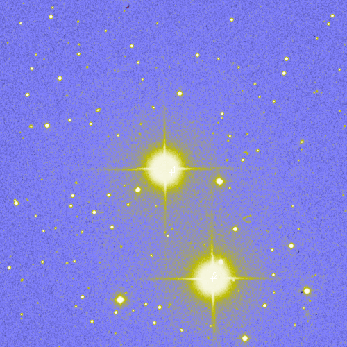
Goddard Skyview Image of 55 Cancri

55 Cancri “A” (the bright star in the middle of the above photo) harbors an extraordinary planetary system. Indeed, it was the subtlety and the depth of the 55 Cancri radial velocity data set that motivated us to develop the systemic console. The fact that the 55 Cancri system continues to defy easy categorization gives us confidence that the systemic collaboration will be a worthwhile project.

Where to begin?

Click on the system menu on the console, scroll down, and select 55 Cancri. (If you’re unfamiliar with the console, and if you’re the methodical type, there are three tutorials available on the menu bar to the right. Otherwise, just follow along!) The published radial data for 55 Cancri now appears in the main console window. The sweeping spray of points, with its curiously non-uniform distribution, contains a fascinating narrative in its own right.

The very first point in the data set has a timestamp of JD 2447578.73 A Julian Date Converter tells us that this was 9:31 PM on Monday Feb. 20, 1989 (Pacific Standard Time). The observation was obtained by Geoff Marcy at the Shane 3-meter telescope at Lick Observatory on Mt. Hamilton, and the velocity error is 9.7 m/s. Back in 1989, Geoff and his colleague Paul Butler were laboring to improve their iodine cell technique, and were struggling to get enough telescope time to adequately track the motion of about 70 nearby solar type stars with the eventual hope of detecting giant planets.

The first 10 radial velocity points were obtained at a rate of 1 to 3 per year. With hindsight, it is easy to see that these 10 points are ample cause for a planet-hunter to be optimistic. The radial velocity variation in the first 10 points spans more than 100 meters per second, suggesting a signal with a signal-to-noise of at least five. The periodogram of these ten points shows a strong peak at 14.65 days, indicating that the data could be explained by a planet with 80% of Jupiter’s mass, circling on an orbit lasting just over two weeks.

Today, if such a planet were discovered, the announcement would not make the news, and the major excitement would be among amateur transit hunters, who would likely have a new high-priority follow-up candidate with a ~5% transit probability. (A two-week period is right at the borderline where transits can be reliably confirmed or ruled out by the photometric collaborators working with the RV-discovery teams prior to announcement of the planet).

In 1993, however, nobody was expecting to find Jovian planets in 14-day orbits. Conventional wisdom at the time was informed by the architecture of our own solar system, and held that gas giant planets should be found beyond the so-called snowline (located at r=4-5 AU) of the protostellar disk. Although the theory of orbital migration had been studied in considerable detail, nobody had proposed that giant planets might regularly spiral in and then be marooned on very short-period orbits. I don’t know whether Geoff and Paul even considered the possibility that the 14.65 day peak in their data was real. If they saw the peak, it is more likely that they would have ascribed it to an alias, an artifact of their uneven hard-won sampling.

During 1994, the velocities suddenly started to trend upward. This would have seemed rather disconcerting, and may even have raised alarm. Was some unaccounted-for instrumental or astrophysical process affecting the newer radial velocity data? Certainly, at the end of 1994, the case for a planet orbiting 55 Cancri would have been weaker than it had been a year earlier.

Nevertheless, the 55 Cancri campaign was at an important turning point. The last measurement of 1994 (JD 2449793.80) has a remarkably lower error (3.3 m/s) than any of the earlier radial velocities. In November of 1994, the Schmidt camera optics on the “Hamilton” spectograph at Lick Observatory had been upgraded, and the resulting improvement effectively tripled the intrinsic resolution to which the spectral lines could be discerned. With the ability to measure radial velocities to a precision of 3 m/s, the planet search had suddenly entered an entirely new realm. When one is in the business of detecting Jupiters, a velocity measurement with 3 m/s precision is literally 10 times as valuable as a velocity with 10 m/s precision.

In October 1995, Mayor and Queloz announced their discovery of a Jupiter-like planet in a 4.5 day orbit around the nearby star 51 Peg. Due to a catalog error that misclassified 51 Peg as a subgiant, it had not been included in Geoff and Paul’s survey, but they were able to rapidly confirm the Swiss discovery.

All at once, the idea of a gas giant with a 2-week orbit was no longer outlandish at all. The telescopes on Mt. Hamilton, which had been slipping inexorably in worldwide prestige as larger telescopes were built on higher mountains, were suddenly at the forefront of relevance. The Lick 3-meter telescope-iodine-cell-spectrograph combination was the best instrument in the world for obtaining precision doppler velocities of bright stars such as 55 Cancri. Extrasolar planets were front page news. Alotments of telescope time increased dramatically. In the six months running from December 1995 through May 1996, 55 Cancri was observed 41 times at Lick. This drastic increase in the cadence of observations is easily visible in the radial data:
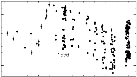
1996 RVs

With the 41 high-quality observations, the presence of the 14.65 day planet was obvious in the power spectrum.
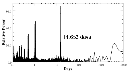
RV powerspectrum

In October 1996, Paul, Geoff, and several other collaborators announced the discovery of the 14.65 day planet, and in January 1997, they published the discovery in a now classic paper that also introduced the world to the inner planetary companions of Tau Bootes and Upsilon Andromedae.

With eight years of data, it was clear that other bodies were present in the system. In the discovery paper, Butler et al. wrote:

The residuals exhibit a long-term trend, starting at -80 m/s in 1989 and climbing to +10 m s-1 by 1994 (the velocity zero point is arbitrary). The velocities appeared to decline toward 0 m s/1 during the past year, although at least another year of data will be required for confirmation. This trend and the possible curvature in the velocity residuals are consistent with a second companion orbiting HR 3522 [aka 55 Cancri] with a period P > 8 yr and M sin i > 5MJUP.

This speculation proved to be correct. Use the console to get a best-fit for the 14.65 day planet, and compute the periodogram of the residuals to the fit:
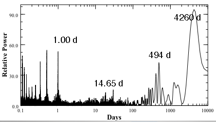
RV residuals powerspectrum

The strongest remaining peak is at 4260 days, corresponding to an 11.7 year orbit (very similar to Jupiter’s 11.8 year orbital period). Keeping the orbits circular, use the “polish” button to produce a Levenberg-Marquardt optimized fit. Zoom in and scroll to show the time interval between 1996 and 2002. The gaps each year when the star is behind the Sun as seen from Earth are easily visible:
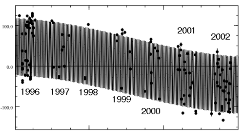
Lick RVs 1996-2002

The two planet system does quite a reasonable (but by no means perfect) job of reproducing the observed radial velocities. After the announcement of the first planet at the end of 1996, interest in the star died down to some degree. The number of target stars being observed at Lick was being increased as Debra Fischer stepped in to manage the Lick Survey, and other systems, especially Upsilon Andromedae, were clamoring for telescope time. During the 1998 season, 55 Cancri was observed only twice. By 1999, however, the Upsilon Andromedae system had been sorted out, and renewed attention was focused on 55 Cancri. During 2000 and 2001, it became clear that the system likely contained at least three planets. With the 14.65 and (in my fit) 5812 day planets removed from the radial velocity curve, the residuals periodogram shows a peak at 44.3 days:
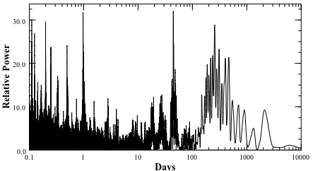
residuals of the residuals

The signal from the 44.3 day planet is not as strong as for the other two planets, but a large number of velocities from 2002 seemed to clinch the case for this third planet:
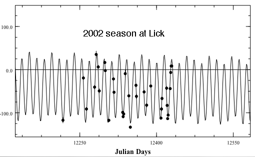
residuals of the residuals

Use the console to optimize the three planet fit using circular Keplerian orbits. When I do this, the chi-square statistic is reduced to 6.4, and the rms scatter is 12.5 m/s. The fit is still not perfect. Either the planets are eccentric, or there are additional planets in the system.

fresh extrasolar planets

fresh extrasolar planets

In a recent article appearing in the Astrophysical Journal, Vogt et al. (2005) published radial velocity data for six stars that appear to harbor multiple low-mass companions. The data for all six stars (HD 37124, HD 50499, HD 108874, HD 128311, HD 190360, and HD 217107) have been added to the system menu of the Systemic Console:
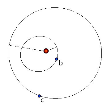
new systems in the console

If you’ve worked through the console tutorials 1, 2, and 3, take a crack at using the console to fit these systems. HD 37124, in particular, is open to several different stable 3-planet configurations. In my current personal favorite fit, three very nearly equal-mass planets are caught up in an endless (or at least multi-billion year) cycle of rub-a-dub-dub. An .mpg animation of the long-term dynamical evolution of the orbits is here. Because the planets in this particular fit are fairly widely spaced, the motion is quite well described by second-order secular theory.

Now fielding three tutorials

Three detailed console tutorials have recently been developed, and are now online at oklo.org.

Tutorial #1 steps through the basic features of the console, using the published radial velocity data-set for the Jupiter-like planet orbiting HD 4208.


Tutorial #2
takes a more detailed look at the console, and shows how to use periodograms and multiple-planet fitting to recover the three planetary companions (the so-called Fourpiter, Twopiter, and Dinky) orbiting Upsilon Andromedae.


Tutorial #3
tackles the tough problem of multiple-planet fitting in the presence of planet-planet interactions, and uses the console to explore the remarkable, recently published Gl 876 data set.

The console has landed.

After more than a year of development work, the beta version of the systemic console java applet is now up and working at oklo.org. Hats off to Aaron Wolf for coding it into reality.

In a series of posts, we will look in detail at the organization, operation, and features contained in the console. For now, however, rev up your G4s and your G5s, take it for a spin, and let us know how it works for you.

The current location for the console is:

www.oklo.org/SystemicBeta/SystemicBeta.html.

It’s also accesible from the menu bar to the right. At the moment it has been tested only with Safari 2.0.2 running on OSX 10.4.3. Firefox 1.0.6 still seems to have issues with the applet. We’ll resolve these first, and then (with CDR Paul Shankland leading the charge) we’ll move on to thwart Bill Gates’ best attempts to protect the MS Explorer user base from Systemic’s seductive charms…

Hello world.

What is systemic?

Systemic is a public research collaboration. Systemic’s goal is to obtain a better understanding of the census of planets in the galaxy.

The systemic blog, hosted by oklo.org, provides a framework for updates and information relating to the collaboration. It also serves as an online forum for discussion of extrasolar planets.