In the posts for Thursday and Friday, we used the Systemic Console to explore the radial velocity variations of 51 Peg. Aside from harboring the first extrasolar planet discovered in orbit around a Sun-like star, this data set is extraordinary because it contains nearly 270 individual radial velocity measurements taken over a period of over ten years. Very few stars have published data sets that are so extensive.

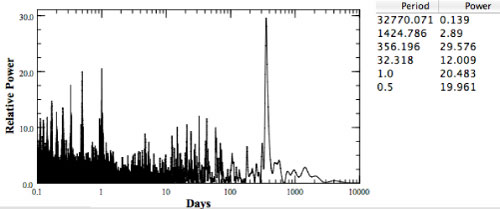
After extracting the signal of the celebrated 4.231 day planet from the data, we computed a periodogram of the residuals. The calculation shows a strong concentration of power at a 356 day periodicity:

At the end of yesterday’s post, we were left hanging on the suggestion that this strong peak might represent a second planet in the 51 Peg system. Let’s have a look at this hypothesis by making a two planet fit to the data.

If you’ve gone through the systemic tutorials, and are comfortable at the controls of the console, here’s the procedure:

Launch the console and follow the directions given yesterday to obtain the best single-planet fit to the data. Next, activate a second planet, and enter 356. into the data window of the period slider for the second planet. Then, minimize the new planet’s mean anomaly, followed by a minimization on the mass. Next, send all ten orbital parameters for the two planets, along with the velocity offsets off for a polish by the Levenberg-Marquardt algorithm. Note that it’s fine to push the “polish” button several times in succession, to ensure that the algorithm has been given enough iterations to converge to the best fit in the vicinity of your choice of starting conditions.

The console shows that the addition of a second planet improves the fit to the data, dropping the chi-square to 1.7, and reducing the required jitter to 5.4 m/s.

The second planet, which we’ll call 51 Peg “c” (where c stands for “console”, huh, huh) has a period of 356.8 days, a minimum mass of 0.32 jovian masses (slightly larger than Saturn), and an orbital eccentricity, e=0.36. Here’s a link to a screenshot of the console showing all the parameters. This is also an advance look at the next version of the console which Aaron will be releasing in a few weeks.

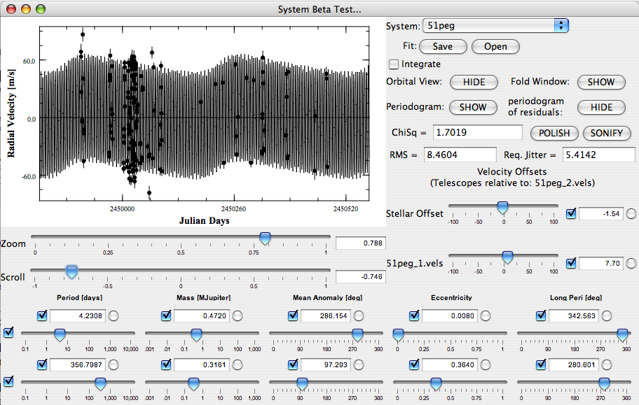
Using the console’s zooming and scrolling sliders, we can see the modulation of the radial velocity curve. The second planet imparts a visibly non-sinusoidal envelope on the strong carrier signal created by 51 Peg b. The non-sinusoidal shape stems from the significant eccentricity of planet “c”:

Note that we still have to teach the console to draw smooth curves when the zoom level is high! Look for that improvement to show up in about 2 months or so. There’s a lot of other items ahead of it on the to-do list.

The orbits of the two planets look like this:

Does it really exist, this room-temperature Saturn? Is it really out there? Do furious anticyclonic storms spin through its cloud bands? Does it have rings? Does it loom as an enormous white crescent in the deep blue twilight sky of a habitable moon?

Maybe.

Eugenio and I have been working through the weekend to devise statistical tests which can assess the likelihood that this planet exists. We’ll check in shortly with our results