
Image Source.
When an extrasolar planet transits its parent star, we get the opportunity to learn the physical size of the planet by measuring how much of the star’s light is blocked during the occultation. To date, fourteen extrasolar planets have been observed in transit, and the big surprise is that they have a much wider range of sizes than astronomers had predicted.
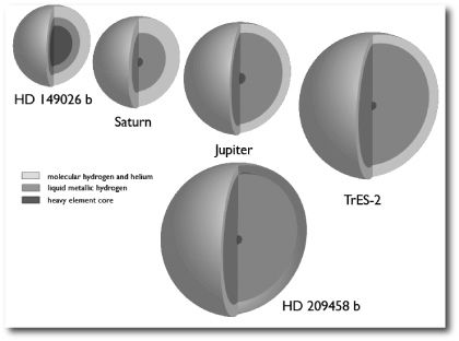
HD 149026 b, for example, is more than 30% smaller in size than one would expect. Its dense, dimunitive stature is thought to stem from a ~70 Earth-mass core of elements that are heavier than the hydrogen and helium that dominate the composition of most of the known extrasolar planets. HD 209458 b, on the other hand, is roughly 30% larger than predicted. The reason for its bloated condition isn’t fully clear, but it’s believed that the planets with larger-than-expected radii are tapping an extra source of internal heat that keeps them eternally buff.
A lot of astronomers are currently interested in the size question for the extrasolar planets, and we’ve written a number of oklo.org posts that cover the subject. [See 1. here, 2. here, 3. here, 4. here, 5. here, 6. here, 7. here, 8. here, and 9. here.]
Josh Winn (MIT) and Matthew Holman (Harvard-Smithsonian CfA) have written a paper that presents an interesting hypothesis for resolving the HD 209458 b radius dilemma. Winn and Holman propose that the planet is caught in a so-called Cassini state, which is a resonance between spin precession and orbital precession. In short, if HD 209458 b is trapped in the “Cassini state 2”, then its spin axis will lie almost in the orbital plane. Like all short-period planets, the planet will spin once per orbit, but it will literally be lying on its side as it circles the parent star. A hot Jupiter in Cassini state 2 will easily experience enough tidal heating to maintain a 30-percent pump.
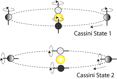
If a planet is in Cassini state 2, then the pattern of illumination on the surface is rather bizarre. At the north and south poles, the parent star rises and sets once per orbital period, and at mid-day passes directly overhead in the sky. This contrasts with the two locations on the equator from which the parent star never rises above the horizon, and the two other spots from which the star never quite sets. Here are two short .avi format animations that help to illustrate the situation. In the first animation, we hover above the point on the equator that receives maximum illumination. In the second animation, we hover above the point on the equator that receives the least illumination.
I’ve been working with UCSC physics graduate student Jonathan Langton to model the surface flows on extrasolar giant planets. As a first research problem, we made simulations of what the surface flows might look like on a planet in Cassini state 2, and compared them with the flows on a planet in Cassini state 1. Jonathan has just had his paper accepted by ApJ Letters. It should show up on astro-ph very shortly, but in the meantime, here’s a link to the .pdf file for the accepted version.
The results of Langton’s simulations are interesting. If the planet is in the standard-issue Cassini state 1, then a steady-state flow-pattern emerges on the planet, with the hottest temperatures occuring eastward of the substellar point, and the coldest region lying near the dawn terminator of the night-side:
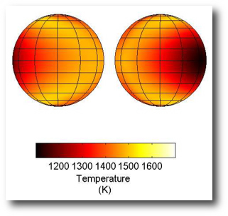
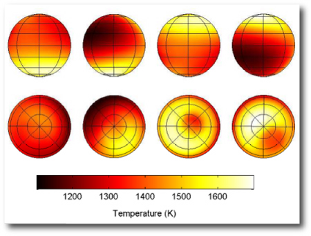
If the planet is in Cassini state 2, then Langton’s model shows that a periodic flow pattern emerges which repeats every orbital period. In the figure below, each successive frame is advanced by 1/4th of an orbital period. The top row of images corresponds to an equator-on view, and the bottom row of images corresponds to a pole-on view:
It’s interesting to watch the animations of the temperature flows. Here’s a link to the equatorial view (5.7 MB, .avi format).
Event though the surface flow patterns are quite different in Cassini State 1 and Cassini state 2, the overall light curves as viewed from Earth don’t show much diffence. The figure below shows infrared emissions from the planet over one full rotation period. The blue line shows the Cassini state 1 light curve, the red line shows the Cassini state 2 light curve. These two curves are more similar to eachother than they are to the Cassini state 1 light-curve predicted by Cooper and Showman (2005), who used a different simulation method and a different set of assumptions, and got a larger overall variation in the predicted infrared emission from the planet during the course of an orbit:
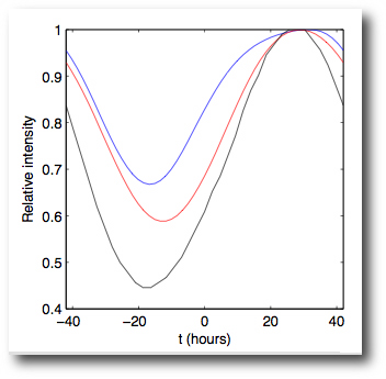
It will be tough to use the Spitzer telescope to reliably distinguish which Cassini State the planet is in.


