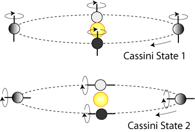
glow

Posted on February 12, 2007 by greg

Saturn reached opposition yesterday, marking the moment in our yearly orbit when the Earth draws closest to the massive ringed giant. At midnight, Saturn is currently the only planet visible in the sky. It’s an odd feeling to stare at the bright unresolved spot of light that encompasses the planet, the rings, and the moons into a tiny golden point, and to know that Cassini, our robot emissary, is actually out there, almost a billion miles away, taking photograph after photograph, and radioing them back to a mere mouse click away.

Saturn and its rings are good reflectors of light, but nevertheless, in the vicinity of the planet, the glare is far from overwhelming. The ambient light levels are only a bit more than 1% that of a bright summer day on Earth. It would be easy to stare at the crisply defined terminator marking the day-night boundary on the planet and the arcs of black shadow cast by the rings. On the Cassini website, there are many views that show the planet as it would appear to human eyes.

Cassini also has the ability to photograph in the infrared. The following false-color photograph shows visible and infrared images of the planet superimposed. In the infrared, Saturn glows with interior heat — still welling up from the planet’s formation — that illuminates the night from within.

The picture above is not a bad approximation of what a younger more massive planet would look like to the naked eye. 2M1207 b, for example, which seems to have a mass about five times that of Jupiter, is in a 1700-year orbit around a young 25-Jupiter mass brown dwarf. At 1250 Kelvin, 2M1207b is still warm enough to be self-luminous in the visible region of the spectrum. It is also slightly illuminated by the light of its companion (whose ~2500K surface is intrinsically 100 times more luminous.) Methane absorption and Rayleigh scattering of incident light in 2M1207 b’s atmosphere likely give the weak crescent a bluish-green hue.

Lonely Planet Guide to the Hyades

Posted on February 9, 2007 by greg

It’s been a hectic week, and now that it’s February, my New Year’s resolution to write 2-3 posts per week managed to lose its shaky option on my priorities.

Eugenio stopped by my office this afternoon to outline his latest code developments for the console. He’s mostly finished implementing a Bulirsch-Stoer integrator. Once this algorithm is tested and operational, it will produce very significant speed-ups for the fitting and the stability analysis of tough multiple-planet systems such as 55 Cancri and GJ 876. Then it’ll be on to a rollout of the bootstrap method for computing uncertainties for the orbital elements in the planetary fits.

“So did you see the new planet?” he asked.

“Huh?” I hadn’t heard anything about it.

Turns out that Bunei Sato and his collaborators have detected a periodic radial velocity variation for the star Epsilon Tauri. Their preprint is on the Astrophysical Journal’s website, but it doesn’t seem to have hit the preprint server yet. This star is a prominent member of the nearby Hyades cluster, and is easily visible to the naked eye as part of the well-known “V”-shaped asterism near Aldeberan in the sky.

Eps Tau is bright enough to have garnered 40 different names in the Simbad catalog, and it’s now listed in the console menu and on the systemic backend as HD 28305. This is one of the most straightforward radial velocity datasets that you’ll come across, and thus makes a good system for first-time users to fit. A few debonair moves with the downloadable console conjure up a model planet with a period of 594 days, an orbital eccentricity e=0.15, and a minimum mass 7.6 times that of Jupiter:

Epsilon Tauri is one of the four stars in the Hyades that are currently nearing the end of their lives and are evolving through the red giant phase. It’s 14 times larger than the Sun, and it’s luminosity is 97 times the solar value. It weighs in at 2.7 solar masses, making it the most massive star known to harbor a planet.

So what’s the story? The Hyades are a metal-rich cluster. One would naively expect that the supersolar composition of the precursor star-forming giant molecular cloud would have lead to a large fraction of the cluster members harboring readily detectable planets. It’s also true that stars somewhat more massive than the Sun should harbor a higher-than-average fraction of giant planets. Eps Tauri scores on both counts.

It’s important to keep in mind, however, that a cluster environment will have a strong effect on giant planet formation. Currently, the Hyades are 600 million years old, and the cluster has lost a large fraction of its O.G.s to the general galactic field through the process of dynamical escape. If we extrapolate back to the cluster’s early days, we find that the Hyades would have resembled the Pleiades 500 million years ago, and would have looked like the Orion Nebular Cluster during the first few million years of its existence.

The UV radiation environment in the original Hyades cluster was fierce. The protostellar disks of the individual Hyads were likely photoevaporated before the growing planetary cores were able to reach the runaway gas accretion phase that gives rise to Jupiter-mass planets (see our paper on this topic). When we get the full inventory of planets in the Hyades, I think we’ll find plenty of Neptunes and terrestrial planets, but almost nothing in the Jovian range. Indeed, work by Bill Cochran and the Texas RV group has demonstrated that the Hyades are generally deficient in massive planets.

My guess is that Epsilon Tauri b is an example of a planet that formed through the gravitational instability mechanism. Gravitational instability should generally produce more massive planets (e.g. HIP 75458 b, and HD 168443 b and c) and its efficacy will be little-affected by UV radiation from neighboring stars. It likely occurs once per every several hundred stars that are formed, and so it’s perfectly reasonable that there’s one star in the Hyades that has a planet formed via the GI mechanism.

a bunch of cool new stuff

Posted on February 2, 2007 by greg

Stefano and Eugenio have both been working hard on the systemic console and backend, and as a result of their efforts, we’re now able to roll out a number of new features.

The backend now features a systemic wiki in which users can collaborate on a wide variety of writing projects related to systemic in particular and extrasolar planets in general. Features include discussion pages for individual systems, the framework for a comprehensive console and backend manual, and an exoplanetary news wire. Our first news service is being provided by Mike Valdez, who combs astro-ph every day and extracts any new preprints that are germane to the those interested in exoplanets. Stefano wrote the code from scratch, so there are endless possibilites for customization. Give it a try.

On the console front, Eugenio has aggregated a uniform listing of the literature sources of all of the radial velocity data sets provided by the console. This information is in a file vels_list.txt, which is now included in the systemic.zip package. If you are using the console for scientific research that you intend to publish, it’s now a snap to get the correct citations for any of the individual systems included on the console.

Many users have expressed interest in what our own solar system would look like to a dedicated radial velocity observer on another star. Eugenio has put together an expansion pack that contains 17 manufactured data sets based on the Solar System. A second expansion pack contains an analogous set of manufactured data sets for various plausible configurations of planets orbiting Alpha Centauri A and B. Both are available on the downloads page for the downloadable systemic console.

Check it out!

…and then the clouds lifted

Posted on January 31, 2007 by greg

I drove up to Berkeley yesterday to give a talk about my second-favorite planet — HD 80606 b. A good fraction of the keynote slides in the talk were new, and so I wound up spending most of the weekend scrambling to get my story straight and to get the talk together.

Pacing is always tricky the first time that you give a talk on a new topic. You’re supposed to practice your talk before you give it, but It’s hard to get in that recommended hour-long practice session when it’s 2AM the night before, and you’re fading, and there are still four slides to finish making.

Thirty-seven minutes into the talk, it suddenly dawned on me that I’d put together too much material, and so I wound up rifling pretty quickly through the last half of the slides. In an entire career as an academic, I’ve never heard of anyone being unhappy when a talk ended on time rather than going over, so I always wrap things up to come in under the bell no matter what.

Over the weekend, I realized a rather remarkable thing about HD 80606b:

Because of the highly eccentric orbit, there’s quite a bit of tidal energy being deposited inside the planet. This tidal energy source, in fact, likely exceeds the amount of energy that the planet absorbs in the form of radiation from the star. For a tidal quality factor, or Q-value of 300,000, the planet will have an effective temperature at apastron of about 390K. That is right at the boundary where water clouds can form in the planet’s upper atmosphere. If the planet is hotter (that is, if Q is lower than 300,000), then the atmosphere will always be cloud-free, and the visible layers of the surface will have a low albedo. If the planet is cooler (that is, if Q is significantly larger than 300,000), then near apastron, the visible surface will consist of a shroud of highly reflective water clouds.

In either event, during the time surrounding ‘606 day, the atmosphere will be too hot for water clouds, and so the albedo will be low when the planet is close to the star. Therefore, if Q is low, there’ll be a smooth variation in the reflected light from the planet over the course of an orbit. On the other hand, if Q is high, then there’ll be a sharp (and potentially observable) drop in the reflected-light signal as the clouds flash to steam.

[I’ve put the slides from the talk on the systemic resources page.]

300B

Posted on January 24, 2007 by greg

The 200-odd extrasolar planets that have been discovered with the radial velocity method are orbiting stars that lie within a few hundred light years of the Sun. The light we now see coming from GJ 876 left that red dwarf back in early August 1991. When you’re in the bars drinking to celebrate the periastron passages of HD 80606 b, it’s easy to forget that last December’s periastron passage actually occurred in September 1817.

By galactic standards, however, a distance of 300 light years is still right next door. For every star within 300 light years of the sun, the Milky Way contains roughly 300,000 additional stars that are farther away. All told, adopting the latest rules on what constitutes a planet, our galaxy likely contains about 300 billion planets, of which perhaps 500 million are hot Jupiters.

Right now, 51 Peg, HD 209458, Upsilon Andromedae, et al. count among the Sun’s local galactic neighbors, but this hasn’t always been the case. The velocity dispersion of stars in the solar neighborhood is ~20 kilometers per second. A kilometer per second is a parsec per million years, which means that in a mere 15 million years, the roster of nearby planets will contain very few familiar names. HD 209458b is transiting now, but in a few hundred thousand years, it’s likely that the line of sight to the system will no longer allow Earthbound observers to watch that dip every 3.5247542 days.

So get out there while there’s still time! Due to a computer glitch, the transitsearch candidates table failed to get its nightly update for the past several nights. I’ve fixed the problem, and the ephemerides are all up to date.

hot and bothered

Posted on January 21, 2007 by greg

When an extrasolar planet transits its parent star, we get the opportunity to learn the physical size of the planet by measuring how much of the star’s light is blocked during the occultation. To date, fourteen extrasolar planets have been observed in transit, and the big surprise is that they have a much wider range of sizes than astronomers had predicted.

Five for the show

HD 149026 b, for example, is more than 30% smaller in size than one would expect. Its dense, dimunitive stature is thought to stem from a ~70 Earth-mass core of elements that are heavier than the hydrogen and helium that dominate the composition of most of the known extrasolar planets. HD 209458 b, on the other hand, is roughly 30% larger than predicted. The reason for its bloated condition isn’t fully clear, but it’s believed that the planets with larger-than-expected radii are tapping an extra source of internal heat that keeps them eternally buff.

A lot of astronomers are currently interested in the size question for the extrasolar planets, and we’ve written a number of oklo.org posts that cover the subject. [See 1. here, 2. here, 3. here, 4. here, 5. here, 6. here, 7. here, 8. here, and 9. here.]

Josh Winn (MIT) and Matthew Holman (Harvard-Smithsonian CfA) have written a paper that presents an interesting hypothesis for resolving the HD 209458 b radius dilemma. Winn and Holman propose that the planet is caught in a so-called Cassini state, which is a resonance between spin precession and orbital precession. In short, if HD 209458 b is trapped in the “Cassini state 2”, then its spin axis will lie almost in the orbital plane. Like all short-period planets, the planet will spin once per orbit, but it will literally be lying on its side as it circles the parent star. A hot Jupiter in Cassini state 2 will easily experience enough tidal heating to maintain a 30-percent pump.

If a planet is in Cassini state 2, then the pattern of illumination on the surface is rather bizarre. At the north and south poles, the parent star rises and sets once per orbital period, and at mid-day passes directly overhead in the sky. This contrasts with the two locations on the equator from which the parent star never rises above the horizon, and the two other spots from which the star never quite sets. Here are two short .avi format animations that help to illustrate the situation. In the first animation, we hover above the point on the equator that receives maximum illumination. In the second animation, we hover above the point on the equator that receives the least illumination.

I’ve been working with UCSC physics graduate student Jonathan Langton to model the surface flows on extrasolar giant planets. As a first research problem, we made simulations of what the surface flows might look like on a planet in Cassini state 2, and compared them with the flows on a planet in Cassini state 1. Jonathan has just had his paper accepted by ApJ Letters. It should show up on astro-ph very shortly, but in the meantime, here’s a link to the .pdf file for the accepted version.

The results of Langton’s simulations are interesting. If the planet is in the standard-issue Cassini state 1, then a steady-state flow-pattern emerges on the planet, with the hottest temperatures occuring eastward of the substellar point, and the coldest region lying near the dawn terminator of the night-side:

If the planet is in Cassini state 2, then Langton’s model shows that a periodic flow pattern emerges which repeats every orbital period. In the figure below, each successive frame is advanced by 1/4th of an orbital period. The top row of images corresponds to an equator-on view, and the bottom row of images corresponds to a pole-on view:

It’s interesting to watch the animations of the temperature flows. Here’s a link to the equatorial view (5.7 MB, .avi format).

Event though the surface flow patterns are quite different in Cassini State 1 and Cassini state 2, the overall light curves as viewed from Earth don’t show much diffence. The figure below shows infrared emissions from the planet over one full rotation period. The blue line shows the Cassini state 1 light curve, the red line shows the Cassini state 2 light curve. These two curves are more similar to eachother than they are to the Cassini state 1 light-curve predicted by Cooper and Showman (2005), who used a different simulation method and a different set of assumptions, and got a larger overall variation in the predicted infrared emission from the planet during the course of an orbit:

It will be tough to use the Spitzer telescope to reliably distinguish which Cassini State the planet is in.

mp3s of the spheres

Posted on January 18, 2007 by greg

New users are still streaming into oklo.org. If you’re a first-time visitor, welcome aboard. You’ll find information that you need to get started in this post from several days ago.

The EZ-2-install downloadable systemic console is the primary software tool that we provide for analyzing data from extrasolar planetary systems. The tutorials 1,2, and 3 are the best way to learn how to use the console. Over the past few months, we’ve been adding a range of new capabilities that go beyond the features described in the tutorials and which improve the overall utility of the software. We’ll be explaining how these new features work in upcoming posts, and for our black-belt users, we’re also putting the finishing touches on a comprehensive technical manual.

When we designed the console, our main goals were to produce a scientifically valuable tool, while at the same time make something that’s fun and easy to use. Early on, we settled on the analogy with a sound mixing board, in which different input signals (planets) are combined to make a composite signal.

We’ve pushed the audio analogy further by adding a “sonify” button to the console. When sonification is activated, you can turn the stellar radial velocity curve into an actual audible waveform. If you create a system with several or more planets, these waveforms can develop some very bizarre sounds. From a practical standpoint, one can often tell whether a planetary system is stable by listening to the corresponding audio signal. Alternately, the console can be used as a nonlinear digital synthesizer to create a very wide variety of tones.

Here are links (one, and two) to past posts that discuss the sonification button in more detail. If you come up with some useful sounds, then by all means upload the corresponding planetary configurations to the systemic back-end.

stability

Posted on January 17, 2007 by greg

If you’re a new visitor to the site, welcome aboard! Yesterday’s post talks about the systemic collaboration, and gives an overview of how you can participate.

The interpretation of radial velocity data sets is confounded by the existence of many different model planetary systems that all do a good job of fitting the data from a given star. If you really want to know whether a particular fit is the correct interpretation of the system, then you need to wait for (or make) more observations to see if your fit’s predicted radial velocity curve is confirmed.

For a real planetary system orbiting a real star, it can take years for enough confirming observations to be made, and so it’s useful to have as many criteria as possible for evaluating whether a particular fit is a contender. Orbital stability provides one such criterion.

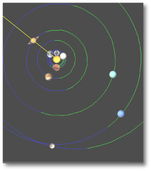
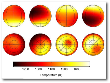
On the backend, there are many orbital models that have been submitted that give excellent fits to the given data sets. For example, the four configurations shown in the picture just below are all acceptable models for the 14 Her system.

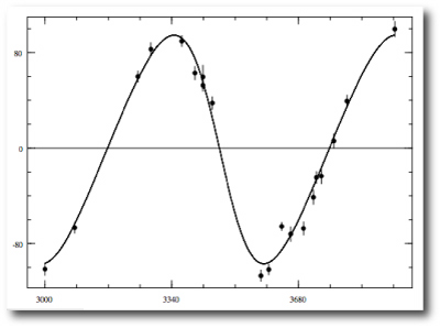
One immediately notices that these orbital configurations look “crowded”. The orbits make close approaches and sometimes even cross. If we let these model systems run forward in time, then we find that the mutual gravitational pulls between the planets lead to catastrophe within a few decades or less. Instead of behaving in an orderly fashion, the orbits execute motions like this:

which lead inevitably to collisions and ejections. While it’s theoretically possible that we happen to be observing a particular system just before it experiences disaster, Occams razor strongly suggests that wildly unstable fits are likely spurious. We can safely exclude any configuration that lasts for only a tiny fraction of the stellar ages (which are generally in the 2-10 billion year range).

Participants in the systemic collaboration can evaluate the stability of their models by using the “check long-term stability” function on the console. Stefano has also recently implemented a robot that crawls through the systems residing in the backend database and integrates all of the submitted fits. So far, it has sorted out which systems are unstable on timescales of less than a century, and as time goes on, it’s pushing the integration times to longer horizons. It turns out that a 100-year integration can catch a majority of the systems that eventually go unstable. After that, we expect roughly equal numbers of systems to be lost in each factor-of-ten increase of integration time.

Although we don’t expect to see orbital instabilities play out on our watch, it’s nevertheless likely that planet-planet interactions and their associated instabilities have played an important past role in sculpting the systems that we now observe. For example, Eric Ford and his collaborators have published a highly plausible theory for the formation of the Upsilon Andromedae planetary system that involves a dramatic instability. In their scenario, the system starts out with four planets, and eventually ejects one of them. The outer two survivors are left stunned and reeling, and the dynamical imprint of the disaster survives to the present day. They’ve made an engaging animation (available here) that shows the action blow-by-blow.

This brings up a relevant question. If orbital instability exists among the extrasolar planets, might our own solar system eventually go unstable? Is it possible that Earth will find itself getting dramatically tossed around the solar system in the manner that was experienced by the unfortunate Upsilon Andromedae E?

The question isn’t new, and the stability of the solar system has been at the forefront of interest for the last 350 years. It was first tackled by Newton, who wanted to understand how the orbits of the Jupiter and Saturn would behave over long periods if their mutual interactions were taken into account. Newton put a lot of effort into the problem, and eventually decided that:

Newton’s fame, and the fact that he’d written off the problem as too difficult, was a big motivation for succeeding generations of mathematicians. Pierre Simon de Laplace eventually solved the problem of the motions of Jupiter and Saturn, and fully explained their orbits to the accuracy that could be observed in the late 1700s. In Laplace’s model, the solar system is completely stable, and the inherent predictability of his planetary motions contributed to the concept of a rational determinism, and the idea of a clockwork universe.

During its first three hundred years, the problem of the stability of the solar system was attacked using pen and paper. In the past few decades, however, the advent of computers has provided a powerful new tool. We can now make accurate simulations of the trajectories of the planets through space, and look in detail at the solar systemâ€™s possible futures. By the 1980s, when hardware and algorithms had progressed to the point were it was possible to integrate the planets millions of years forward into the future, it was found that the solar system is chaotic in a sense originally envisioned by PoincarÃ©. If the position of a planet, the Earth say, is given a tiny change in the computer, then as millions of years elapse, this slight perturbation grows erratically larger. If Earth is displaced in its orbit by a centimeter, then, after several million years, Earth will likely be located somewhere within 2 centimeters of where it would have been had it been given no push at all. After several million years, the degree of uncertainty doubles again, this time to 4 centimeters.

Worrying about such tiny buildups of uncertainty in the position of Earth on its orbit sounds utterly absurd. Nevertheless, like interest compounding in a forgotten account, the accumulation of uncertainty is guaranteed to eventually become significant. After a hundred million years, which is much less than the 4.5 billion year age of the solar system, the position of Earth in its orbit becomes completely impossible to predict. For times 100 million years in the future, we have no firm knowledge of Earthâ€™s trajectory. We have no idea whether January 1, 100,000,000 AD will occur in the winter or in the summer, or even whether Earth will be orbiting the Sun at all.

PoincarÃ©â€™s great insight was that the realistic physical description of non-trivial systems can involve what we now call chaotic behavior. The weather is an excellent example. Overnight weather forecasts are generally quite accurate. Three-day forecasts are certainly of some utility. Two-week forecasts, on the other hand, are essentially worthless. Although we have a very clear understanding of the laws of physics that govern the behavior of Earthâ€™s atmosphere, we can’t sample global weather conditions with enough precision to make forecasts accurate beyond a few days. If you let out a deep sigh at the complexity of it all, then the air current that you exhale will spur subtle deviations in the flow of air and moisture of the Earthâ€™s surface that become increasingly magnified over time. The aggravated swirl of air from a slap at a mosquito can career into divergences that visit a hurricane on Miami rather than spinning it out into oblivion over the North Atlantic. Although we canâ€™t accurately predict how the pattern of weather fronts and daily high temperatures will look on the 10:00 p.m. News two weeks from today, we do have some idea of what the weather will be. If it is in the middle of the summer, Texas will be hot. Duluth, in January, will be cold. The pattern of erratic day-to-day weather is superimposed over solidly predictable seasonal and regional climates.

We can thus ask the question: Are the movements of the planets predictably chaotic in the same sense as the weather? That is, over billions of years, will the planets wander only within circumscribed bounds, or is a more wild chaos, with orbit crossing, ejections, collisions and the like â€“ a real possibility?

The answer will be a statistical statement. To high probability, the planets will remain more or less on their present courses until the Sun becomes a red giant. Exactly how high a probability is not fully clear. Stay tuned…

Armchair Planet Hunting

Posted on January 15, 2007 by greg

The Associated Press just published an article on how the Internet has facilitated an increasing number of collaborations between amateur and professional astronomers. The systemic project is one focus of the AP piece, and we’re seeing a jump in traffic as a result. If you are a first-time visitor to the site, welcome aboard!

There are several ways that you can use and participate in systemic. Our project home page is a weblog (updated fairly frequently) that gives an insider’s perspective on the latest developments and discoveries in the fast-moving fields of extrasolar planets and solar-system exploration. We write for a target audience of non-astronomers who are interested in astronomy. To get a flavor for the blog, keep reading the posts below, or have a look at a few of our past articles, such as our take on last Summer’s big “is Pluto a planet debate”, our exploration of what planets and galaxies really look like, or our series [1, 2, 3, 4] on the feasibility of detecting habitable terrestrial planets in the Alpha Centauri System.

You should see a set of links just to your right:

These links give you information that you can use to start participating in the actual discovery and characterization of extrasolar planets. (Despite the fact that we’re rocket scientists, we’ve been unable to consistently sweet-talk Microsoft IE into correctly displaying our site. On some versions of IE, you may have to scroll all the way down to the bottom of this page to see the links). The Downloadable Systemic Console is our Java-based software package that allows you to work with extrasolar planet data. The Systemic Backend is a collaborative environment that has the look and functionality of a social networking site. Registration and participation are free. The nearest well-characterized extrasolar planets (GJ 876 b, c and d) are 14.65 light years away, and so the news of useful modern innovations such as pop-ups and spyware hasn’t had time to propagate to those far-distant worlds. Hence the systemic backend is completely free of annoying ads!

One final note: there are two separate channels for registration on systemic. The first, accessed through the “login” tab on the site header above, is part of the WordPress package that runs the blog. Registration on the blog allows you to comment on our frontend posts. The second, accessed through the “backend” tab on the site header or the link to the right, gives you access to the collaborative php-based environment that constitutes the systemic backend. You can register for either or both, and you don’t need to give your real name or any real-world identifying information other than an e-mail address.

Tune in regularly for more news and updates.

So Which Planet is on Your Coffee Table?

Posted on January 10, 2007 by greg

Image Source.

Newly published high-profile books get set out prominently on the display tables at the front of Borders in downtown Santa Cruz. During this past holiday season, one of the prime spots was given to Postcards from Mars by Cornell’s Jim Bell, who is the Pancam lead scientist for NASA’s Mars Exploration Rover Mission. The book is superbly produced. The Pancams’ high resolution allows the photos in the fold-out spreads to convey an impact that’s hard to achieve by surfing the NASA website with your browser.

With all the focus on Mars, I think the public tends to forget that Cassini, NASA’s flagship mission, is sending back an even more amazing trove of images from a far more alien environment. Indeed, Jeff Cuzzi (a colleague from my NASA Ames days) along with Laura Lovett and Joan Horvath, have just written a coffee-table book, Saturn A New View, that highlights the most stunning images of the Saturnian system. At the moment, the book is buried back in the science section at Borders, but it absolutely deserves a spot out in front as well. The “upgrade”, if you will, from Voyager to Cassini is an order of magnitude more impressive than the jump from Viking to Spirit and Opportunity.

I was nine years old when Viking 1 landed on Mars in 1976, and I vividly remember seeing the first images of the martian surface on the CBS morning news. I also recall that I was quite interested when the Voyagers sent back the first close-ups of Saturn and its environs, but I can’t remember the exact moment of seeing those photos for the first time. A quarter century later, this same gap in enthusiasm is reflected by the fact that the Mars book has an Amazon sales rank that is way ahead of the Saturn book.

On Mars, when you look at the landscape, the scene is familiar. It looks like a rocky desert on Earth. In the mind’s eye, you can place yourself on the surface. You can imagine hiking into the hills on the horizon. In short, you know what you’re seeing.

Image Source.

With Saturn, on the other hand, the views are abstract and alien. We don’t have rings in our sky, and so I’m intuitively unfamiliar with the play of shadows on the surface of the planet and the rings. When you look at views of Saturn, there’s no sense of being “right there”. You have to think more carefully to really see what you are seeing.

Image Source.

It amazes me that the size of Saturn and its rings is quite comparable to the Earth-Moon distance. Using Illustrator to superimpose the Earth and the Moon on the Saturnian system, the scale looks like this:

It took the Apollo astronauts about a day to traverse a distance equivalent to the diameter of Saturn. (It took them three days to make the trip from the Earth to the Moon.)

From Earth, when Saturn is visible overhead at midnight, it lies about 8.5 AU away. This means that the diameter of the A-ring subtends about 3/4 of an arc minute in the sky. That’s somewhat below the resolution limit of the human eye. If Saturn lay at Jupiter’s distance, however, people with sharp eyes would just barely be able to distinguish it as appearing slightly oblong.

Until I read the new Saturn book, I had not realized that the northern hemisphere of Saturn currently appears blue. It’s winter in Saturn’s northern hemisphere, and the tilt of the rings blocks additional sunlight from reaching the upper half of the planet. The frigid conditions have caused the ochre-colored haze to dissipate, and we have a view down to the methane-rich red-absorbing regions at greater depth. It’s the same effect that gives Neptune and Uranus their blue cast.

Billions of years from now, after the Sun has turned into a white dwarf, and after the planets have lost the majority of their internal heat, all four giant planets will take on the blueish color that Neptune and Uranus currently have. The current color of Saturn’s frigid northern hemisphere is an early preview of things to come.