Looks like Geoff Marcy won the is-Pluto-a-planet debate. His stylish quote (reminiscent of Pablo Picasso’s comments to the New York Times on the occasion of Apollo 11) dramatically wrapped up Dennis Overbye’s NYT article, and made the whole brouhaha look rather foolish indeed.

I’ve been trying to take the high road too, but so far with no success. This morning, I succumbed to temptation and jumped into the fray by way of Rob Roy Britt’s cnn.com piece, snidely pointing out that eccentric satellite orbits can sometimes lead to the satellite being promoted to a planet for part of the orbit and demoted to a mere moon for the remainder:

Higher resolution version here.

Then, less than an hour later, I was talking to a departmental colleague about scientifically useful questions, when our conversation suddenly fell into the Pluto trap. We spent an enjoyable half-hour batting around a comfortably well-worn sequence of conversational bon mots. My colleague — an eminent planetary scientist — was pleased to take a tough-guy approach: Eight planets. He’s in favor of a 10-year phase-out for Pluto, now that the New Horizons probe is on its way and (presumably) safely beyond the grasp of NASA budget cuts. We agreed that a decade is more than enough time to give the kids’ plastic placemat manufacturers and textbook publishers enough time to switch the production lines over to the correct version of the solar system.

With the circulation of Alec Wilkinson’s recent New Yorker piece, planet placemats and mobiles have emerged as a topic of discussion. In Kitchenport, in downtown Santa Cruz, there are indeed plastic placemats for sale featuring the eight inner planets and Pluto. I was surprised to find Saturn listed as the “slowest planet” on the mats:

This inspired me to one-up my colleague with an even tougher-guy approach: Take a historically stringent view and limit the planets to the five classical wanderers of the heavens, thus dramatically restoring Saturn to its rightful position as the slowest planet.

Bob Naeye over at Sky and Telescope has been blogging the planet debate as well. He caught an arithmetic error in the original version of yesterday’s post. In my haste to slap the post up on the blog, I used da/dt=.374 cm/yr rather than the correct value of da/dt=3.74 cm/yr in the timescale estimation.

A first estimate for the Moon’s promotion timescale can be made with the following logic. The Moon becomes a planet when the distance to the moon is such that the Earth-moon barycenter lies at the surface of the Earth. The barycenter of the orbit at that time will be defined by

with Rm being the distance from the Earth to the Moon. The system mass ratio is

According to the IAU draft resolution, the Moon will turn into a planet at the exact moment when the barycenter moves above the surface of the Earth, which is located at R=6.378e+8 cm. Assuming a circular orbit, the Moon thus needs to be at a=5.18e+10 cm, which means that the Moon needs to recede from its current orbital radius by da=1.34e+10 cm. At the current rate of da/dt=3.8 cm/yr, this would take 3.5 billion years, a timescale that is well within the life expectancy of the Earth in the face of possible destruction by the Red Giant Sun.

This is just a first approximation, however. In reality, the time will be considerably longer, both because the tidal force (and hence the dissipation) decreases as the moon goes outward, and because the current rate of tidal dissipation is near a geological maximum, most likely because the Earth’s oceans are presently in a near-resonant, highly tidally dissipative configuration.

Assuming a constant value of the tidal quality factor Q, the time interval T, required for a satellite to recede from an initial orbital radius a_i to an orbital radius a_0 is given by

In the above, k_2=0.299 is the Earth’s Love number. Currently, Q=12 for the Earth. Plugging numbers into the above equation yields a time T=1.57 billion years for the Moon to recede to its current location. In the past, however, the average value for Q was higher, and it is likely that it will also be higher in the future. Given that the age of the Earth-Moon system is 4.5 billion years, average Q for the Earth has been more like Q=34. If we assume that Q=34 holds as a long term average value, then we arrive at a best estimate of T=26.8 billion years until the Moon is promoted to planetary status.

Sadly, though, the Moon’s reign as a planet will ultimately be limited. Planetary status is achieved when the Moon’s distance reaches 81.3 Earth radii. For the next 23 billion years thereafter, the Moon will be living the bling planetary lifestyle as it slowly continues to recede. When the Moon reaches ~87 Earth radii, the length of Earth’s rotation will have decreased to ~47 days, and the Earth and the Moon will be tidally despun. Thereafter (as described by Jeffreys, 1970), tidal interactions between the Earth, the Moon, and the Sun’s remnant white dwarf will drive the Moon back inward, eventually stripping it of planetary status, and finally destroying it by tidal breakup into a massive ring system.

You guys have all read about the recommendation of the IAU committee.

Looks like the Moon’ll be a planet soon! Tidal evolution is currently driving it outward at 3.74 cm per year. It appears that the Moon will be admitted into the planetary club in roughly 30 billion years if we aren’t destroyed by the Sun’s Red Giant phase.

I’m almost too young to remember the Apollo missions. I was five years old in December 1972. Despite great protests and resolve, I had long since gone to bed when Apollo 17 blasted off in a dramatic night launch that marked the last journey into deep space. Early the next morning, Bobby Robinson came running breathless to our back door, “They’re showing the countdown again on TV!” We sprinted down the block through the cold to his house, bursting into the den. The brilliantly spotlighted Saturn V was still on the launchpad. “Four Three Two!” Billows of flame filled the screen. The slow, almost imperceptible lift-off. Shards of ice condensed from the humid Florida air fell away from the great frozen missile like waterfalls.

For days afterward, we built rockets out of legos.

One of our recurring goals here at oklo is to gain an accurate idea of what the extrasolar planets really look like. We’re working on this by connecting detailed numerical simulations to state-of-the-art rendering. The photographs brought back by the Apollo missions provide a key basis of insight into much of what we can expect to see. Inspired by Michael Light’s Full Moon, I’ve thus been spending time working through the Apollo Lunar Surface Journal, which provides a detailed commentary and a near-complete trove of images and video from all of the lunar missions. It’s easy to become engrossed to the point where hours simply disappear.

Several impressions hang in my mind. When Earth is in view, or when you’re standing on the airless lunar surface with the Sun at your back, the sky is completely black. No stars visible, no glowingly luminous nebulosity in the sky. The dynamic range vastly exceeds what the human eye can handle.

If the Sun is in view, light scattered by the optical system — be it a Hasselblad camera lens, or a gold-plated faceplate visor, or an eye lens — has a huge effect on the visual field. An understanding of the lens flare is essential to producing a realistic visual impression.

Harrison Schmitt aboard Apollo 17

When the Apollo Spacecraft arrived at the Moon, one astronaut remained alone aboard the command module, in orbit a mere 65 miles or so above the lunar surface. For the half of each orbit above the lunar farside, radio communication was impossible, with the signal regained each time the Earth rose above the horizon.

Ken Mattingly, of Apollo 16 described the experience of being alone in orbit:

I was lying there, looking out the window as we moved across the terminator. I was listening to the Symphonie Fantastique, and it was dark in the spacecraft. I was looking down at dark ground, and there was Earthshine. It was like looking at a snow-covered Earth scene under a full moon.

Image Source.

Unless lightning strikes, the lower layers of the Earth’s atmosphere contain very small fraction of charged particles. The air is electrically neutral, and indeed is a fairly good insulator. This state of affairs is something to be thankful for.

Imagine what would happen if the air started to carry a tiny ionization fraction. That is, imagine if one out of every million air molecules were stripped of an electron. The ionized air molecules and the electrons would experience an immediate desire to spiral around the Earth’s magnetic field lines. In doing so, they would bash into the surrounding sea of neutral particles and drag them along with their motion.

Bulk motion of charged particles drags magnetic field lines along and vice-versa. Magnetic field lines, however, don’t like being compressed or twisted, and have a tendancy – verging on insistence – to spring back into shape. If the Earth’s atmosphere had a small magnetic field, the jet stream would rapidly wind up the Earth’s magnetic field, which would angrily resist the winding and pull backward on the jetstream. Our normal weather patterns would be thrown into complete and utter disarray.

In the inner regions of a protostellar disk, the temperature is high enough for trace elements such as sodium to lose their outer electrons. This raises the ionization fraction of the disk gas to the point where the ambient magnetic field begins to play an important role. This, in turn, leads to an interesting situation.

Imagine two parcels of disk gas on a circular orbit. Imagine also, that the two parcels are connected by a weak magnetic field line. Next, perturb the leading parcel by pulling backward on it slightly. Such a pull drains orbital energy from the parcel and causes it to drop down to a lower orbit. A lower orbit, however, has a faster rotational velocity. The faster rotational velocity causes the parcel to run forward. This pulls on the magnetic field line, which pulls back, forcing the particle even further down into the gravitational well. Clearly, we have the condition for a runaway situation.

This process, known as the magnetorotational instability was discussed by Chandrasekhar in the late 1950’s, and appears in his monograph on Hydrodynamic and Hydromagnetic Stability, and was brilliantly revived in the context of disks in the early 1990’s by Steve Balbus and John Hawley. The nonlinear outcome of the magnetorotational instability is turbulence in the disk. This turbulence may play an important role in allowing mass to slip down and accrete onto the star.

The magnetorotational instability is a simple consequence of the remarkable fact that self-gravitating systems have a negative heat capacity. Balbus and Hawley completely cleaned up by recognizing the importance of the instability within the context of accretion disk physics. Their 1991 paper has now garnered 960 citations. I’m of the opinion that there may be some similarly useful gems ready to be mined out of several of Chandrasekhar’s more opaque books. In fact, I’m going to put on my mining helmet and stake some claims inside of Ellipsoidal Figures of Equilibrium.

HD 80606 b is one crazy place. With an orbital eccentricity of e=0.932, its orbit resembles a ball tossed almost straight up with a 111.4 day hang time. I’ve heard that in many European countries, periastron passage (when HD 80606 b whips through its closest approach) is known as ‘606 day, and is celebrated by a day off work filled with drunken and disorderly parades. I’m trying to bring the tradition over to the United States.

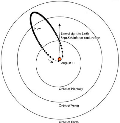
Today (as viewed from Earth) HD 80606 b is just starting to pick up speed on its inward plunge to the next ‘606 day, which occurs on August 31, 2006. The planet has spent the June and July cooling off near the far point of its orbit, at a distance of about 0.85 AU from the central star. It’s possible that weather in the upper atmospheric layers of the planet has spawned a street of category 10 hurricanes that will tear unimpeded around the planet until the steadily mounting insolation turns the driving rains into steam. During the month of August, the planet will fall in almost the full distance to the star, eventually swooping within 6 stellar radii as it whips through periastron.

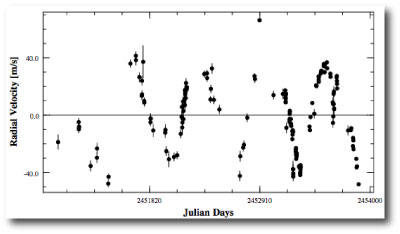
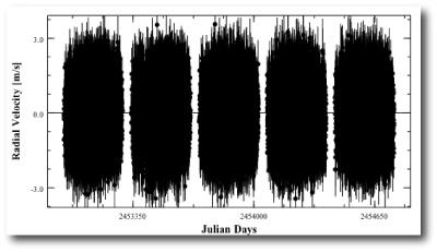
The discovery of the planet and its orbital solution were announced by the Geneva Observatory Planet Search Team in an April 04, 2001 ESO press release, and the radial velocities are available on both the downloadable systemic console and at the CDS repository (see Naef ef al 2001). The recent catalog paper by Butler et al. (see exoplanets.org) tabulates an additional set of 46 high quality velocities for HD 80606. Using the console to get a joint fit to the two datasets gives an updated set of orbital elements: P=111.4298 days, M=3.76 Jupiter masses, and e=0.9321.

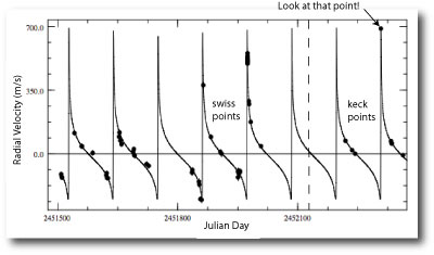
Several years ago, when the California-Carnegie radial velocities for HD 80606 started coming in, Geoff let me have an advance look at them. When I synched the new Keck points up against the Swiss points (which I’d extracted from a published postscript figure) I noticed something interesting. The Keck point obtained on Feb. 2, 2002 was more than 100 m/s above a cluster of Swiss velocities that had been obtained very close to periastron passage.

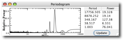
I got excited. The Keck observation suggested that the magnitude of the periastron swing is larger than had been estimated by the published fit. This in turn suggested that the eccentricity of the planet was even larger than the published value of e~0.93. I did an orbital fit and uncertainty analysis on the combined dataset. The best-fit eccentricity came out at a whopping e=0.971 +/- 0.018. An eccentricity this high implied that the planet was regularly swooping to within 2.5 stellar radii of the star. In order for this to be possible, the so-called tidal Q for the planet would have to be very high — higher than the value of around a million that had been inferred from the orbital circularization radii for the hot Jupiters.

In order to confirm the high eccentricity, it would be necessary to obtain more radial velocity measurements in the vicinity of the periastron swing. In June of 2004, I calculated a list of the upcoming periastron dates, and found that one was scheduled for July 11th, 2004 (UT), just a few weeks away. I looked at the schedule for the Keck I telescope, and saw that the California Carnegie team had been assigned a run covering July 8th, 9th, 10th, 11th and 12th. Then I checked where HD 80606 would be located in the Mauna Kea sky. The star was setting rapidly, and was already fairly far to the west at sunset, with and hour angle of more than five hours, and airmass of about three.

I wrote to Geoff and told him about the combined fit that suggested a high eccentricity. Would the star be high enough above the horizon for Keck to observe? He wrote back right away. He was also computing a high value for the eccentricity, and yes, it would be within the limits of observability if the telescope operator was notified in advance.

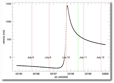
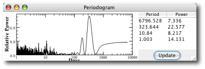
In the plot just above, I’ve reproduced the predicted radial velocity curve during the course of the run. The four vertical red lines show 8:00 PM Keck time on July 8th, 9th, 10th, 11th, and 12th, 2004. Amazingly, the fit suggested that during the brief window of observability on July 10th local time (July 11th UT), the star would be smack in the midst of its most rapid acceleration! The radial velocity fit suggested that a standard six-minute exposure started at 07:30 PM on July 10th would span a reflex velocity change of 60 m/s. By contrast, it takes Jupiter 6 years to indude a 12 m/s velocity change in the Sun.

I waited impatiently through the run, eager to learn what the velocities would be. I kept my fingers crossed that the eccentricity would hold up at e=0.97. Money in the bank. Even if the velocities drove the eccentricity down to its 1-sigma low bound, to e=0.953, it would still be an exciting result, with potentially important consequences for the internal structure of the planet.

On July 10th, at 11 pm PDT (8 pm Hawaii time) I sat at my kitchen table, and imagined the scene on Mauna Kea, with the great dome open to the sky, and Keck I leaning practically on its side, straining to catch the rays of a distant star fading into the last moments of twilight. I thought of the planet itself, stellar furnace filling half the sky, literally jerking the star back into space as it screamed through periastron.

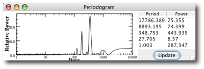
On the morning of the 13th, Geoff sent an e-mail with the velocities. The new fit gave e=0.945. I was stunned. What the @#%? I looked at the velocities themselves, On the 10th, on what was supposed to have been big night, the velocity had failed to rise at all from the value on the 9th. On the 11th, the velocity was only somewhat higher. It was clear that the big swing had occurred several hours afterward. On the 12th, the velocity was high, and clearly past the peak. The planet had arrived at periastron slightly more than a full day later than predicted.

The measured eccentricity was 2-sigma low, an occurrence that one expects less than 2.5% of the time. By chance, the high Keck velocity on Feb. 2, 2002 randomly came within one part in 2000 of arriving exactly at the radial velocity maximum. The fitting program interpreted this high point as suggesting a higher eccentricity than the planet actually has.

I was depressed for the next fifteen minutes. As usual, 95 to 97% of the “cool” discoveries that one turns up in the course of scientific life turn out to be spurious. You have to keep throwing your hat into the ring.

For a theorist, the path of least resistance leads to the abstract. I start to think of planets as signal-to-noise, as peaks on a periodogram. As grant proposals come due, as manuscript drafts bounce back and forth between editors, authors and referees, it’s easy to forget that the planets are really out there, falling endlessly through empty space.

On Monday, we drove up to the Lick Observatory. From the hot rush-hour smog of I-680 in downtown San Jose, the summer-yellow folds of the Diablo range rise out of the hazy valley air. The white telescope domes cling to the highest ridgeline. Exit at Alum Rock. Drive several miles east. The city thins out into suburban sprawl. The Mt. Hamilton Road starts just at the point where the mountains begin to slope up steeply. It takes nearly an hour to cover the 19 miles to the summit, where the observatory buildings sleep mirage-like in the quiet sunlight. Hawks circle against the blue sky. The grasses have dried to straw, and the heat draws the smell of sage and pine resin into the still air.

The dome of the Automated Planet Finder is in place now, and the telescope is nearing completion. It’s visible just to the right of the larger three-meter dome in this photo taken from the main observatory building. The Automated Planet Finder will produce long strings of precise radial velocity measurements. Very soon, we’ll be posting synthetic data sets on the systemic back-end that mimic the observational cadences that this telescope will be capable of providing. It will detect some very interesting planets.

The 36-inch refractor, housed in the great dome of the main building, is still in perfect working order, but it has long since ceded it’s relevance to the cutting-edge. In 1892, E. E. Barnard used it to discover Amalthea, the tiny fifth satellite of Jupiter. This was the last moon in the Solar System to be discovered with the naked eye. More than a century later, the telescope waits silent and unused through most nights. The body of James Lick lies interred at its base. Crickets, lodged in unseen corners of the old building, chirp intermittently in the dark.

Support astronomer Bryant Grigsby brought the great refractor to majestic life. To locate an object on the sky, he repeatedly executed a delicately choreographed sequence of maneuvers. The dome must be rotated so that the slit is positioned on the correct part of the sky. The giant polished and inlaid wood floor must be raised or lowered by up to 16 1/2 feet to bring the eyepiece to eye-level. The 25,000 pound, 57-foot long telescope, perfectly balanced on its pivot, is pulled by hand into rough position, followed by a series of fine adjustments to bring the target into view. The great refractor is priceless. If it’s broken or rendered inoperable, it won’t be replaced. Bryant told me that it took many nights to acquire the confidence to maneuver it on his own.

Just before midnight, he swung the telescope low, nearly to its declination limit, and brought Neptune into view. In the high-power eyepiece, it swam, a dim, very pale, bluish-white circle cut out against matte black. Several star-like points were in the field. One of them may have been Triton. Using Illustrator, I’ve tried to capture how it looked.

What I can’t fully capture, though, is what it is like to stare, for long unhurried minutes, at a giant frigid world on the fringe of our Solar System, with the crickets chirping in warm dry quiet of the dome, illuminated faintly by the glow of a low-watt red bulb and a window open to the distant twinkling lights of the city grid.