Image Source.

It was a brilliantly clear November afternoon today, and the fact that the Sun’s rays were diminished by 0.0026% mattered not one jot. Mercury was in transit.

I was fortunate to get a glimpse of the event through a telescope. It was about an hour before third contact, and Mercury was clearly visible as a tiny, perfectly round, perfectly black dot set against the pale yellow immensity of the solar disk. There was something about the simplicity of the situation that was quite striking.

Transits, with their odd cadences, link the timescales of human activity to the flow of astronomical time. The June 2004 transit of Venus, for example, took place on the day before the final exam for my introductory Astronomy class. In the weeks leading up to the exam, I would point to Venus shining in the early evening sky, and urge the students to study, “See how it’s getting noticeably lower in the Sky every night at sunset? You can use the angular distance between Venus and the Sun as a countdown clock to the final!” (At which point they’d roll their eyes.)

The next Venus transit is in 2012. The one prior to 2004 took place in 1882, when William Harkness wrote,

We are now on the eve of the second transit of a pair, after which there will be no other till the twenty-first century of our era has dawned upon the Earth, and the June flowers are blooming in 2004. When the last transit season occurred the intellectual world was awakening from the slumber of ages, and that wondrous scientific activity which has led to our present advanced knowledge was just beginning. What will be the state of science when the next transit season arrives, God only knows. Not even our children’s children will live to take part in the astronomy of that day. As for ourselves, we have to make do with the present.

Accurate weather predictions are good for no more than a few days, but transit predictions can be made a long time in advance. For example (according to the Wikipedia) simultaneuous transits of Mercury and Venus will occur in the years 69163 and 224508.

Motions in the inner solar system are nevertheless chaotic, though, with a Lyapunov timescale of order several million years. Our lack of absolutely precise knowledge regarding the positions of the planets at the present moment gradually exponentiates into much larger uncertainties. As a result, we can predict transits millions of years into the future, but we have no ability to predict when the transits of hundreds of millions of years from now will occur.

In fact, there’s even a (thankfully small) chance that the solar system will become dynamically unstable before the Sun swells into a red giant. This afternoon, Mercury seemed utterly insignificant and completely remote when pitched against the solar disk. In the final hours before a collision with the Earth, however, it would present an altogether different sort of impression.

Good news for the systemic user base! Eugenio has posted a new version of the downloadable systemic console. This most recent update fixes several bugs, and offers a better graphical interface for those working at limited display resolutions. Progress overall has been rapid during the past several days, and next week we’re planning to roll out both a fully threaded version of the console as well as the Systemic Jr. catalog of synthetic radial velocity data sets. Systemic Jr. will be a testbed for the full Systemic simulation, and will allow us to answer a number of interesting questions regarding the fidelity of planetary models as a function of orbital parameters and observational sampling. Put oklo.org on your bookmark list and tell your friends to drop by. We’ve manufactured plenty of consoles to hand out.

By tomorrow I’ll be back on the extrasolar planets beat, but I thought it would be interesting to show a few more results connected to the strange orbits detailed in the previous post.

It’s clear from the sample of eight orbits that were charted that the m=1 singular isothermal disk potential supports an extensive variety of orbital families: tube orbits, box orbits, chaotic orbits, resonant orbits, and Enron orbits just to name a few. Is it possible to design a map that shows the regions of parameter space that are delineated by the different kinds of orbits?

The best method that I’ve been able to devise consists of what I’ll call an “excursion map”. We can clasify orbits by the total angle that they accumulate over time. For example, a loop orbit (such as the first trajectory shown in the previous post) experiences a steady accumulating of total angle — 360 degrees worth per orbital period. A box-type orbit on the other hand (like the seventh and eighth trajectories shown in the previous post) oscillates back and forth across the x-axis and never accumulates more than 90 degrees or so of total angular excursion. Chaotic orbits (such as the sixth example trajectory) execute a random walk in angular excursion, and on average accumulate a total absolute angular excursion (either positive or negative) which is proportional to the square root of the time.

We can thus pack information about the orbital structure of the potential function into a single diagram. We choose intial starting conditions parameterized by position on the x-axis and the e-parameter of the potential function. A given starting condition corresponds to a point on a two-dimensional diagram, and also defines an orbit. The orbit can be integrated for a characteristic time (t=1000, say) and the total angular excursion or the orbit can be logged. A color code can then be assigned: white for orbits that accumulate positive angle in direct proportion to the time, gray for orbits that accumulate angle in proportion to the square root of the time, and dark gray for orbits that never get beyond plus or minus 90 degrees. With this coding, the excursion map looks like this:

The numbers label the locations of the 8 different orbits shown in the previous post.

Take orbit 3, for example. It corresponds to a loop-type orbit within an island of similar loop orbits surrounded by a sea of chaotic orbits. If we zoom in on the island with a magnification factor of ten, we see structure emerge. Tiny changes in the initial conditions determine whether an orbit is stable (white) or chaotic (gray). Two jagged fingers of box orbits jut up into the map.

Zooming in by another factor of ten shows that the map has a fractal structure, with detail emerging on every level of magnification:

It’s strange to realize how so much bizarre structure is inherent within such a simple potential function. Somehow, encapsulated into one simple formula, the dynamics are all folded up like an inifinite series of orgami cranes, waiting patiently to be observed…

Image Source.

The academic quarter is pulling up to the half-way point at UCSC, and it’s getting tougher to keep up with everything that I’m supposed to do. I’ve been spending a lot of time getting the lectures together, so in the interest of sticking to a schedule of posts, I thought I’d veer from the all-planets-all-the-time approach and show some scanned transparencies from Friday’s class.

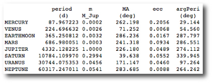
The orbit of an idealized planet around an idealized star is a keplerian ellipse. A planet on an elliptical trajectory conserves its eccentricity, orbital period, longitude of periastron, inclination, and line of nodes. The only orbital element that changes over time is the mean anomaly. We can thus say that the Keplerian orbit contains five integrals (constants) of the motion.

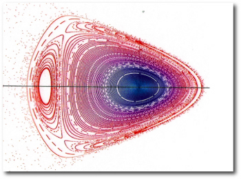
If the potential arises from a mass distribution that’s not a perfect point mass, then in general we won’t have five integrals of motion. It’s interesting to look at a subsection of the weird variety of planar orbits that occur in a two-dimensional potential distribution that looks like this:

The ln(r) term causes this potential goes to negative infinity at the origin while remaining unbounded at large radii. The second term, in which e is specified to take on values between 0 and 1, lends a modulation that makes the force law non-axisymmetric with respect to the origin. One can roughly think of orbits in this potential as the motion of a marble rolling in a funnel-shaped, lopsided bowl.

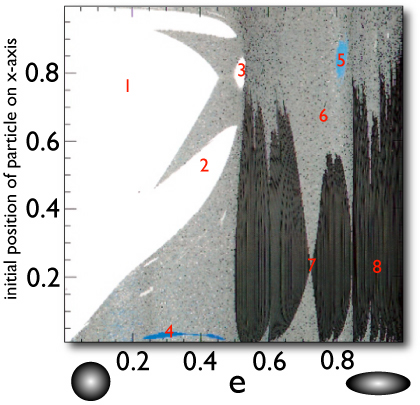
The potential function does not change with time, and so the energy of an orbiting particle is conserved. Further, because of the self-similarity of the potential, the structure of orbits at one energy will be an exact copy of the orbit structures at all other energies. Thus, there’s no loss in generality by sampling orbits having only a single total energy (kinetic + potential). In the following sampler of pictures, I integrate the trajectories of single particles launched from the long (+x) axis of the potential with initial velocities always perpendicular to the long axis. The magnitude of the velocities are determined by the total energy choice: particles starting closer to the origin must have a higher initial kinetic energy to offset their more negative gravitational potential energy. I also vary the parameter e.

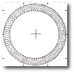
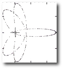
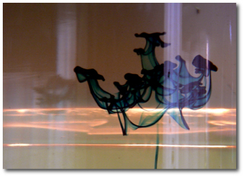
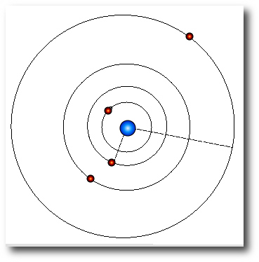
For e=0.2 and an initial position x=0.78, the orbit is reasonably circular, and steady precession smears the excursion of the particle over many orbits into a thin annular region centered on the origin.

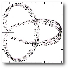
For e=0.42, x=0.55, the particle starts fairly close to its zero velocity curve. It thus falls inward almost to the origin before making a second loop, and then a second approach to the origin which sends it rocketing back up close to its initial position.

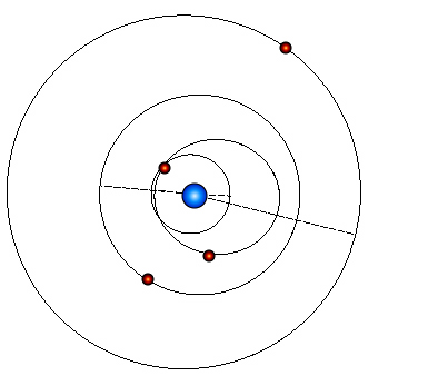
Taking e=0.2, x=0.78 leads to a single loop orbit that dives in very close to the origin.

Here’s the result of taking e=0.42 and x=0.55. It’s a good thing the Earth isn’t orbiting in this potential with these particular starting conditions.

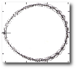
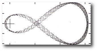
This one, which arises from e=0.81 and x=0.85 is pretty cool. Most of the time it runs counterclockwise as viewed from above, but before close approach to the origin it switches to clockwise. One’s tempted to classify it as an Enron orbit. From all appearances it appears to be clocking a steady increase in angle, whereas in reality, when the books are finally audited, it’s accumulating -2pi radians every period.

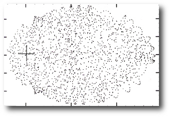
Choosing e-0.30, x=0.03 launches the particle on a highly chaotic trajectory. This orbit is uniformly sampling the entire area allowed to it by its total energy constraint.

For larger values of the e parameter the orbits often show a fundamentally different behavior. Choosing e=0.72, x=0.22 leads to a motion which is restricted to oscillations of a narrow angular range centered on the long-axis of the potential. The particle is basically rolling back and forth in the narrow valley provided by the high-e potential.

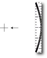
e=0.90, x=0.20 gives an orbit with a similar quality: