Screen-Shot-2013-04-07-at-4.44.18-PM

This was no fruit of such worlds and suns as shine on the telescopes and photographic plates of our observatories. This was no breath from the skies whose motions and dimensions our astronomers measure or deem too vast to measure. It was just a colour out of space—a frightful messenger from unformed realms of infinity beyond all Nature as we know it; from realms whose mere existence stuns the brain and numbs us with the black extra-cosmic gulfs it throws open before our frenzied eyes.

H.P. Lovecraft, The Colour out of Space Amazing Stories, Vol. 2, No. 6 (September 1927), 557–67.

I’ve always thought that the Colour out of Space was H.P. Lovecraft’s best effort. One can argue about economy of expression, but the story is nearly unmatched in its attempt to confront — and imagine — the truly alien.

I think we currently have substantially less understanding of the extrasolar planets than is generally assumed. Thousands of planets are known, but there is no strong evidence that any of them bear a particular resemblance to the planets within our own solar system. There’s always a tendency, perfectly encapsulated by the discipline of astrobiology, with its habitable zones and its preoccupation with water — to make wild extrapolations into the complete unknown.

An interesting synopsis of much of what we do know can be gained by looking at the latest mass-radius diagram for the exoplanets. The number of planets with joint mass and radius determinations is growing rapidly, and the elastic virtue of a log-log plot fails to suppress the huge range in apparent planetary structures. To within errors, it appears that 6-Earth Mass planets range in radii by a factor of at least three. This is impressive, given that constant density implies R~M^{1/3}…

Screen-Shot-2013-04-07-at-4.11.08-PM

On the figure, I’ve plotted three potential mass-radius relations for super-Earths. This first (in Earth units) is the standard-issue M=R^{2.06} fit that one gets from the solar system planets (excluding Jupiter). The second (again in Earth units) is the vaguely alarming M=3R relation suggested by Wu & Lithwick’s transit timing analysis. The third mass-radius relation is what one might expect if planets form in-situ and accumulate low-density hydrogen envelopes around rocky cores. (Evaporative mass loss makes this more of an upper limit). Frustratingly, all three relations remain plausible.

It’s thus fantastic news that NASA’s TESS Mission has been selected for flight. TESS will find effectively all of the transiting Super-Earths orbiting the few million brightest stars, and with dedicated ground-based radial velocity follow-up, will — less than a decade from now — allow for a fantastically detailed version of the above plot.

The Tau Ceti Five

Screen-Shot-2012-12-19-at-10.45.51-AM

Tau Ceti has street cred. Lying only 11.9 light years away, it is the second-closest single G-type star. It’s older than the Sun, and photometrically quiet. It’s naked-eye visible from both hemispheres, ensuring VIP seating at any SETI fundraiser.

And so what about planets? It’s been clear for a few years that Tau Ceti has a zeroth-order dissimilarity with the solar system. That is, if it had a Jovian-mass planet in a Jovian-like orbit, a press conference would have been dedicated to it several years ago. Indeed, because it is so bright and so quiet, Tau Ceti is among the handful of stars in the sky that are best suited to long-term high-precision monitoring via the Doppler velocity technique. It’s at or near the top of the list for all of the major Doppler surveys.

Tau Ceti displays a marked excess luminosity in the far-infrared. Blotchy sub-millimeter images imply that this excess luminosity arises from a wide ring of cold dust at Pluto-like distances from the star. In this picture, the radiating dust arises from ongoing collisions within a Kuiper belt-like disk comprising roughly an Earth-mass worth of icy asteroidal bodies:

Screen-Shot-2012-12-31-at-10.45.37-AM

Tau Ceti’s Kuiper belt seems to be about ten times more massive than our own Kuiper belt, despite the fact that Tau Ceti’s metallicity is only about one-third that of the Sun. There’s little risk in hypothesizing (read hand-waving) that the low metallicity of Tau Ceti’s protoplanetary disk meant slow growth for Tau Ceti’s retinue of proto-Jovian cores, which subsequently missed out on rapid gas accretion. The ensuing presence of Neptunes, and the concomitant absence of a Jupiter, generated a different dynamical history compared to the Solar System’s — namely one with more stuff left over at the end of the day in the icy outer reaches.

Given this picture, the a-priori odds are excellent that Tau Ceti resembles tens of billions of ordinary, single Population I stars in the galaxy and also harbors multiple inner planets with masses between Earth and Neptune, on nearly circular, nearly co-planar orbits with periods of 100 days or less. Should such worlds exist in orbit around Tau Ceti, then it’s likely that sufficient radial velocity data now exist to dig them out…

Readers surely noticed the paper by Mikko Tuomi and colleagues that was posted to astro-ph earlier this month. Tuomi and collaborators report on a joint analysis of three large-N data sets that comprise thousands of radial velocity measurements (from HARPS, KECK and AAT) spanning a total time base line in excess of 13 years. Ideally, one would like have a fully definitive conclusion emerge from such a massive data set, but frustratingly, Tau Ceti is holding its cards very close to the vest, and as radial velocity half-amplitudes inexorably drop below K=1 m/s, this will be an increasingly common behavior from other nearby high-value stars. In their arXiv preprint, Toumi et al. lay off their risk and remain ambiguous regarding actual detections of actual planets, providing only a fully hedged speculation at the end of the abstract, that these “periodicities could be interpreted as corresponding to planets…”

The modeling strategy for Tau Ceti taken in the Tuomi et al. paper provides an alternative to the approach adopted by Dumusque et al. in digging the K=0.5 m/s Alpha Cen Bb out of a similarly challenging data set. For both systems, the authors adopt the stance that it is no longer sufficient to write off excess scatter in radial velocity fits as “stellar jitter”. Dumusque’s team developed a physical model for starspot activity migrating latitudinally on a differentially rotating star, and also modeled the convective blueshift arising from stellar activity. Application of these physical models spurred the removal of systematic “noise” from the time series, thereby revealing a candidate Earth-mass planet in a 3.2-day orbit. Tuomi et al. excavate five potential planets by exploring the use of ARMA(p,q) — AutoRegressive Moving Average — models which recognize that (in addition to a Keplerian signal) both the value of given velocity measurement as well as its accompanying error are potentially correlated with previous measurements. ARMA models and their generalizations, ARCH, GARCH, NGARCH, etc., are an old standby for modeling financial time series. Near-term VIX predictions anyone?

Indeed, planet detection and trading have certain similarities. Noisy signals, non-stationary processes, cut-throat competition, and the opportunity to land yourself in the media spotlight when things go awry.

And the possible planets? Should the signals isolated by Tuomi et al turn out to be both real and Keplerian, then Tau Ceti will join the legions of stars in the galaxy that harbor fully ordinary planetary systems.

TauCeti6

The MMEN

Galileo’s unveiling of Io, Europa, Ganymede and Callisto is unarguably shortlisted for the most important astronomical discovery of all time. The Galilean satellites constitute a planetary system in miniature, and their clockwork presence is a centerpiece of Newton’s De mundi systemate.

And indeed, if one bases one’s expectations for exoplanetary systems on the Jovian satellites (as well as the regular satellite systems of Saturn and Uranus) then the startling abundance of compact systems discovered by the Geneva Team and by Kepler are hardly startling at all. The Galaxy’s default planetary system — as expressed around many, if not most of its stars — has a handful of planets on near-circular orbits, with periods ranging from days to weeks, and masses of order one part in ten thousand of the central star. Out here in the sticks, near the Sun, we’ve got an Earth, yes, but unlike most stars, we have no super Earths.

There is an intriguing, seemingly anti-Copernican disconnect between the solar system and the extrasolar planets. Much of the theoretical framework of planet formation is based on the paradigm provided by the Minimum Mass Solar Nebula (MMSN), the $\sigma \propto r^{-1.5}$ disk of net solar composition that is required to account for the solar system’s planets. In the standard formulation, the MMSN holds its power-law form inward to about 0.5 AU, where it meets a murkily indistinct inner boundary that’s needed to account for the lack of anything interior to Mercury’s orbit.

Interestingly, the MMSN fades out just where the super-Earths really start to appear. This has led to the widespread assumption that planets somehow form at large radii and then migrate long distances in order to be found in their observed orbits. That seems rather odd.

Eugene Chiang and I have been exploring an alternative idea — namely that the solar system doesn’t present a good starting template for studying extrasolar planets, and that planets, in general, don’t migrate very far (if at all). Could it be that the huge population of super-Earths formed right where they are observed? If that’s the case, it makes life simpler, and it implies that the template we’re after is the Minimum Mass Extrasolar Nebula (MMEN), which can be defined by grinding up the planets that have been observed by Kepler, and which is not all that different from what one gets if one simply takes the MMSN and runs it all the way into the dust sublimation boundary at ~0.05 AU.

Our paper is available at arXiv.

The Crescent Neptune


A few weeks ago, I got an e-mail from a reporter related to a story that will feature favorite space photos:

We’re hoping some space-themed photo comes to mind, either a picture taken by a space telescope, or by yourself from your own backyard, or anything else that relates to space. We’d also welcome any comments about the photo’s meaning to you.

I think my favorite space photo is the Voyager image of the crescent Neptune and Triton.

For two reasons. First, there’s no false color, no artifice, no agenda. This photograph is calming, mysterious and aesthetically perfect.

Second, the image is dominated by the night side of Neptune. Implicit in the photograph is the amazing fact that it was taken from a vantage that was further than the Sun than the planets. Less than one Neptune orbit elapsed between its discovery in 1846 and the Voyager flyby in 1989. A crescent Neptune seems to me far more subtly profound than the iconic “pale blue dot” image taken by the same spacecraft not all that long thereafter.

Alpha Centauri B b


Image Credit: ESO.

I had the good fortune of being asked to sit in as an external commentator for the ESO’s media briefing on the Geneva Team’s discovery of Alpha Centauri B b. It was startling to see the amount of interest on the line. All of the familiar names from the science journalism community were logged in, and there was a very substantial representation from the mainstream media. The ESO officials remarked that it was the largest audience that they’d ever seen for a press briefing. It was very clear that Alpha Centauri and Earth-mass planet combine for a headline draw. The story was supposed to be held until 17 Oct. 19:00 CET, but the embargo was broken in rather disorderly fashion, and, according to ESO, b, by the end of the afternoon was officially out of the bag.

Paul Gilster, who leads the Centauri Dreams site asked me for a brief perspective for a piece that he’ll be writing tomorrow (Lee Billings has a very nice article on Centauri Dreams today). I was eager to oblige — Paul has played a clear, consistent role in getting the community’s attention focused squarely on or charismatic next-door neighbor. I wrote back:

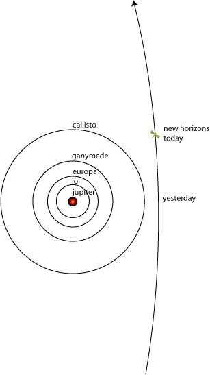
I really like the particular way that the narrative is unfolding. The presence of the 3.2-day planet, taken in conjunction with the myriad Kepler candidates and the other results from the HARPS survey, quite clearly points to the possibility, and I would even say the likelihood, of finding additional planets at substantially more clement distances from the star. Alpha Cen A and B, however, are drawing closer together over the next several years, severely metering the rate at which high-precision measurements can be obtained. This builds suspense! It reminds me a bit of a mission like New Horizons, where the long coast to the destination serves to build a groundswell of excitement and momentum for the dramatic close encounter. I think that this is important for a society that is increasingly expectant of immediate interactivity and instant gratification… I hope that this detection of Alpha Cen Bb provides an impetus for the funding of additional radial velocity infrastructure, and also for space-based missions such as TESS, which can find and study the very best planets orbiting the very nearest stars.

With K=0.51 m/s, Alpha Cen B b has a RV half-amplitude that is over a third lower than the previous record-holder, HD10180b. The relative insignificance of an Earth-mass world in comparison to the great bulk of Alpha Cen B is immediately evident with a scale diagram of the star, the orbit and the planet. The planet resolves to ~6/10th of a pixel in this figure, barely visible as a faint gray speck.

As far as the faint gray speck itself goes, the ESO-produced artist’s impression (shown as the splash image for this post, and over the past few hours, splashed all over the Internet) is quite good for this genre. Granted, the apparent surface brightness of the Milky Way in the background is about 1,000,000,000 times too high, but the planetary crescent and the lighting geometry make the grade. And thankfully: No lava.

Alpha Cen B has a radius about 90% as large as the Sun. This means that transits, if they occur, would have a maximum photometric depth of ~0.01%, and would last up to three hours. These numbers make for a challenging, but by no means impossible, detection. HST (perhaps using the FGS instrument) should be able to reach a transit of this depth, and given that the phase, the depth, and the period are known in advance, I think that a purpose-engineered ground-based solution can be made to work as well. For example, see this post on orthogonal transfer arrays — Alpha Cen B delivers almost 5 megawatts to the Earth, and Alpha Cen A is a nice comparison star right next door.

During the press briefing, the “habitable zone” came up repeatedly. Put succinctly, Venus at B would be on the A-list.

The Nature News and Views commentary by Artie Hatzes draws on the extraordinary claims argument to imbue the detection with a question mark. “The researchers used 23 parameters related to the star’s rotation period to model the variation in stellar activity, and then filtered it out from the data, unveiling the planet’s signal.” Given the skepticism, it’s interesting to look in more detail at how the signal was dug out.

In the past, I’ve used this blog as a platform for urging that Alpha Cen receive the maximum possible allotment of Doppler-based attention. From August 2009:

Now nobody likes backseat drivers. As the saying goes, “theorists know the way, but they can’t drive”, and theorists have had a particularly dismal record in predicting nearly everything exoplanetary.

But nevertheless, I’m urging a factor-of-four increase to that data rate on Alpha Cen B. I would advocate two fully p-mode averaged velocities per night, 50 nights per year. I know that because Alpha Cen B is so bright, the duty cycle isn’t great. I know that there are a whole panoply of other interesting systems calling for time. It is indeed a gamble, but from the big-picture point of view, there’s a hugely nonlinear payoff in finding a potentially habitable planet around Alpha Centauri in comparison to any other star.

The current HARPS data set has an impressive 459 individual p-mode averaged velocities, with uncertainties in the range of 1 m/s. In a naive universe governed by featurelessly luminous stars and normal distributions, such a data set would allow planetary orbits with K<0.1 m/s to be probed. It was just such a universe that informed some of my earlier simulated data sets that modeled what one might expect from Alpha Centauri. For instance, here’s a plot from June 2009 that shows what I thought the HARPS data set of that time might have looked like.

With 459 points along such lines, Alpha Cen’s whole retinue of terrestrial planets would now be visible. Indeed, with just the synthetic data in the above figure, a simulated super-Earth in the habitable zone sticks out like a sore thumb.

With hindsight, it’s not surprising that the real data set is more complicated. Although Alpha Cen B is a very quiet star, it does have a magnetic cycle, and it does have starspots, which rotate at the ~37-day spin period of the star, and which come and go on a timescale of months.

The raw radial velocities are completely dominated by the binary orbit. The following figure is from the SI document associated with the Dumusque et al.’s Nature article.

Alpha Centauri B has a velocity component in our direction of more the 50,000 miles per hour, more than twice the speed attained by the Saturn V’s just after their trans-lunar injection burns. The AB binary orbit has a period of ~80 years, and is currently drawing toward a close approach on the planet of the sky. (Figure below is from Wikipedia.) The next periastron will be in 2035.

Strictly speaking, one needs five parameters (P, K, e, omega, and MA) to model a binary star’s effect on a radial velocity curve. However, because the HARPS data covers only 5% of a full orbit, it’s sufficient to model the binary’s contribution to the Doppler data with a 3-parameter parabola. When the binary is removed, the data look like this:

There’s a clear long-term multi-year excursion in the velocities (traced by the thick gray line), and there are almost 10 meters per second of variation within each observing season. That’s not what one would have ideally hoped to see, but it is an all too familiar situation for many stars that have years of accumulated radial velocity data. Browsing through the Keck database shows numerous stars with a vaguely similar pattern, for example, this one:

Many long-term trends of this sort are the product of stellar activity cycles that are analogues of the 11-year sunspot cycle on our own Sun. In the absence of sunspots, the surface of a sun-like star is uniformly covered by granulation — the pattern of upwelling convective cells.


Image Source.

Most of the surface area of the granules is composed of plasma moving up and away from the Sun’s center. The gas gushes upward, disgorges energy at the photosphere, and then spills back into the darker regions that delineate the granule boundaries. On the whole, the majority of the stellar surface is blueshifted by this effect. In the vicinity of sunspots, however, the granulation is strongly suppressed, and so when there are a lot of sunspots on the surface of the star, the net blueshift is reduced.

Sunspot activity is very tightly correlated with the strength of emission in the cores of the Calcium II H and K lines (for an accessible overview, see here). As a consequence, a time series of this so-called H&K emission is a startlingly good proxy for the degree to which the granulation blueshift is suppressed by sunspots. Figure 2 of the Dumusque paper charts the H&K emission. Its variation is seen to do an excellent job of tracking the erratic long-term Doppler RV signal displayed by the star (compare with the plot above). Hence, with a single multiplicative scale parameter, the variations measured by the H&K time series can be pulled out of the Doppler time series.

Can’t stop there, however. Starspots, which come and go, and which rotate with the surface of the star at the ~37-day stellar spin period, generate an additional signal, or rather sequence of periodic signals and overtones. Dumusque et al. handle the rotation-induced signals in conceptually the same way that one would handle a set of planets with variable masses, periods of several months: measure the strength of the periodogram peaks, and remove the signals year by year. This involves 19 free parameters, the moral equivalent of successively removing four planets to get down to the final brass (or more precisely iron) tack:

The Pythagorean Problem

Image source: Drew Detweiler

The Pythagorean version of the gravitational three-body problem is very simple to state.

Assume that Newtonian Gravity is correct. Place three point bodies of masses 3, 4, and 5 at the vertices of a 3-4-5 right triangle, with each body at rest opposite the side of its respective length. What happens?

This particular problem seems to have been first posed in the late 1800s by the German mathematician Meissel, who mysteriously asserted that the motion of the three bodies should be periodic. That is, he felt that they would come back to their exact starting positions after executing a complex of intermediate motions. A first attempt at the solution — using numerical integration with a variable stepsize — was published in 1913 by Carl Burrau. He was able to map out the intial trajectories through several close encounters, but he was unable to integrate far enough to determine what eventually happens.

The correct solution was found in 1967 by Szebeley and Peters, who used the technique of three-body regularization to resolve the succession of close encounters. Here’s one of their diagrams showing a segment of the complicated motion.

The Szebehely-Peters paper is fun to read. It emphasizes that this nonlinear problem is surprisingly tricky to solve, and that it shows the classic sensitive dependence on small variations in the initial conditions. For example, here’s a link to a recent, attractively rendered YouTube video that animates the trajectories and osculating orbits, as obtained via an implementation that uses Mathematica’s NDsolve.

Screenshot source.

Unfortunately, however, a careful analysis shows that the motion from 2:47 through the end of the video is completely incorrect…

I’ve always been struck by the fact that there’s a fascinating subtext to the trajectories of the three bodies if they are interpreted as a narrative of interpersonal relations. An initial value problem for a set of six coupled, first-order ordinary differential equations unfolds to telegraph a drama of attraction, betrayal, redemption, triumph and loss.

This summer, I had an opportunity to collaborate on the development of a scored, choreographed 3-minute 45-second performance of the problem which was premiered last month at the ZERO1 Biennial in San Jose. Our goal was to simultaneously convey the interpretive subtext while adhering to an fully accurate set of trajectories. It took a lot of work and was quite an intense experience. From the description at the ZERO1 site:

Three dancers in illuminated costumes create a live video visualization of the elliptic-hyperbolic solution to the classic Pythagorean three-body problem. A custom light tracing application detects light emitted from LEDs on the dancers’ soft circuitry costumes to create a visual model of their trajectories across the 2D plane of the stage. This realtime graphic visualization is projected on a large screen behind the stage in order to provide the audience with a birds eye perspective of their complex motion.

The use of digital technologies presents challenges for contemporary choreographic methods as data visualization guides movement through performative space on scientifically accurate trajectories. Live accompaniment from three musicians enhances physical performance as each body is interpreted through movement and sound. Feelings of longing, connection, and isolation are intertwined as the bodies are flung apart by the same gravitational forces that draw them together.

(That last sentence could more properly read, The bodies are flung apart despite feeling only attractive gravitational forces.)

To give a better sense, here are some notes and diagrams from mid-way through the process, as the choreography and the rehearsals were beginning to gel.

It’s particularly fascinating how the immediate outcome of the near-return to the pythagorean condition at the halfway mark is so different from how things unfold at the start of the piece. I like the interpretation that body 4 is somehow lazy at this point, or late to realize the import of the situation, and is marginalized as a result. This is the first real opportunity for bodies 3 and 4 to express emotion — shock for body 4, joy for body 3.

In the following measures, body 4 is marginalized, sulky, scheming, whereas body 3 is doing its best to impress, in the set of looping, private engagements. A reverie! The successive body 3-5 interchanges should _highlight_ the difference in masses between 3 and 5. Body 3 is light footed, fleet, body 5 glides smoothly, deliberately, (but not dully) as an anchor.

Body 4 must come back from its runout with a renewed sense of determination and purpose. The ensuing encounter between 4 and 5 must somehow convey 4’s charms and strengths. In a very real sense, this encounter is the tipping point that determines the outcome for all time. This is where the youtube video went off the rails.

As a consequence, there should be a sense of unfulfillment in the next body 3-5 encounter (a grasp, a gaze that fails to connect?) which sets up 3 to dive through on the way to its penultimate run-out. In this sequence, body 3 must somehow fail to live up to the expectations that it so brightly promised. The outcome is now determined, and the bodies know it, although the audience doesn’t.


While body 3 is at the arc of its final run-out, body 4 is weaving a spell on body 5, cementing the outcome ever more decisively. Indeed, Body 5 is only briefly engaged as 3 makes its final dramatic run through body 4 and 5’s orbit. The final sequence of encounters between body 4 should grow ever more identical, signaling the finality of the outcome.

The latest anomalies

Photographed at UCSC Art Dept. Spring 2012 Open Studios

The announcement of new transiting hot-Jupiter type planets, such as WASP 79b or HAT-P-38b, by the ground-based surveys no longer generates press releases, but the march of discovery does give us an ever-clearer view of the planetary census.

Yesterday, Matteo Crismani turned in his UCSC Senior Thesis. In addition to the results that we published in our 2011 paper (described in this post and this post) he also took an updated look at the relationship between the radius anomaly (the fractional discrepancy between the theoretically predicted radius and the actual observed radius) and the insolation-derived effective temperature of the planet. With the large aggregate of hot Jupiter-class planets that now have good measurements for both planetary mass and planetary radius, the dependence of the radius anomaly on the planetary temperature has grown clearer.

The best fit power-law now has the radius anomaly scaling as T^2.9, with an uncertainty on the exponent of ~0.3. This is quite close to the T^2.6 relation that stems from the back-of-the-envelope arguments that invoke the Batygin-Stevenson Ohmic heating mechanism. In effect, these hot Jupiters are like Ball Park Franks…

11 December, 2117

Full-size (1536×2048) .gif images: one, two.

We went up to Mount Hamilton yesterday afternoon, and, as was the case for everyone who saw the transit, it was a unique conjunction of time, place, and circumstance.

The Lick Observatory staff deployed the historic 36-inch refractor to extraordinary advantage. Rather than project the image, which has the effect of divorcing the instrument from the event, they removed the eyepiece and stretched a cloth across the focal plane. The resulting effect, somehow, was to seamlessly integrate the transit into its surroundings and its historical context, 1639, 1761, 1769, 1874, 1882, 2004, 2012…

Headed out to Pluto

Time slips by. It’s now been more than six years since launch and more than five years since the New Horizons probe got its gravitational assist from Jupiter. I looked back through the oklo.org archives and found a post covering the event.

One day, one hour, and nine minutes ago, the New Horizons spacecraft sailed flawlessly through its closest approach to Jupiter. A day later, Jupiter still looms large in New Horizon’s field of view, with an angular size more than five times greater than the size of the full moon in our sky.

That was on March 1st, 2007, a day after the 500 point drop in the DJIA that signaled the first shudder of unease portending the global financial crisis.

Oklo.org and New Horizons have both been gradually slowing down over the past six years, with New Horizons passing the orbit of a planet at roughly the cadence of 100 additional oklo posts. New Horizons is currently 9 AU from Pluto, and will arrive in the system in July 2015.

I discovered from reading the wikipedia page that a third circumbinary satellite was recently found in orbit around Pluto and Charon.

The three small moons in the Plutonian system are surprisingly reminiscent of what we might expect a typical circumbinary extrasolar planetary system to look like: orbital periods measured in weeks, masses of order a part in ten thousand of the central binary, low eccentricities, and orbits that are close to, but not in mean-motion resonance. During the next few years, as the Kepler data continues to roll in, and as the eclipsing binary systems in Kepler’s field of view are carefully scrutinized, we’ll find out whether such properties are indeed the norm.