Sonified

Many systemic readers have not yet experienced the thrill of fitting planetary systems with the systemic console because the console fails to properly launch in their browser. The standard refrain for the last several months has been, “We’re working on it…”

Tomorrow, we’ll be releasing an upgraded version of the console in downloadable form. We’ve tested this version on Mac OSX, Windows, and Linux platforms, and we’ve gotten it to work on all three.

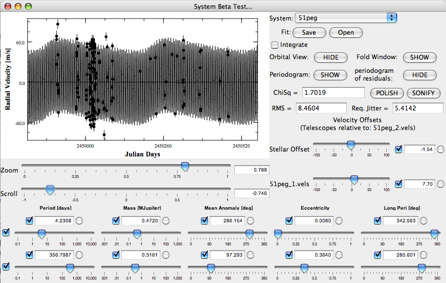
The downloadable version of the console will contain a number of new features, including a sonification button that brings up the following window:

console sonification controller

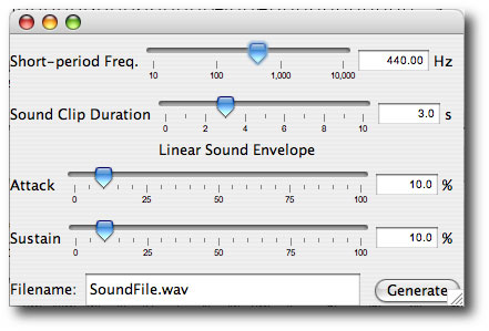
Sonification takes the N-body initial condition corresponding to the current positions of the console sliders and performs an integration of the equations of motion to produce a self-consistent radial velocity curve for the star. The radial velocity curve is then interpreted as an audio waveform and the resulting audio signal is written to the .wav format. You, the user, choose the duration of the integration and the audio frequency to which the innermost planet’s orbital frequency is mapped (440 Hertz, for example, corresponds to the A below middle C). A simple envelope function is also provided in order to avoid strange-sounding glitches associated with sharp turn-on and turn-off transients.

A single planet in a circular orbit produces a pure sine-wave tone. Very boring. The introduction of orbital eccentricity adds additional frequency content to the single-planet signal, and produces a variety of buzzing hornlike timbres, depending on the chosen values for the eccentricity and longitude of periastron. (For example, here are tones corresponding to keplerian orbits with [1] e=0.5, omega=90 deg; [2] e=0.9, omega=150 deg; and [3] e=0.9, omega=312 deg).

Hewitt, Conceptual Physics, p. 284

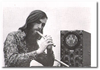
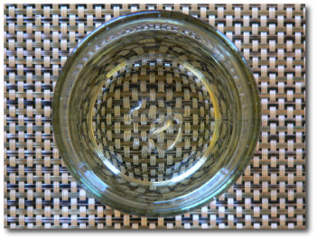
I scanned the above photo from my groovy 1974 edition of Conceptual Physics. Author Paul Hewitt is using a pipe to generate what looks to be a 420 Hz tone. The oscilliscope trace indicates that the pipe is producing both a fundamental frequency as well as a first overtone. A similar effect can be had with the console by adding an additional planet and sonifying the resulting radial velocity curve. For example, a quick fit to the 55 Cancri data-set generates a flute-like timbre that arises primarily from the near 3:1 commensurability of the orbits of the 14.65 and 44.3 day planets. Here’s a detail from the waveform:

55 Cancri Waveform

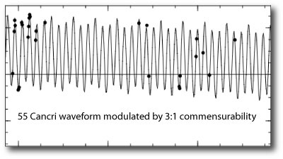
And here’s the .wav format audio file corresponding to the 55 Cancri fit.

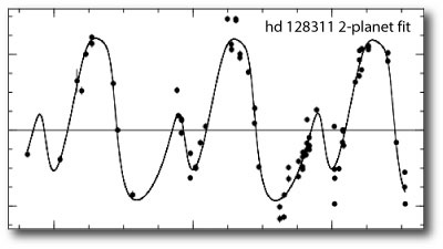
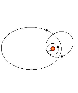
Systems in 2:1 mean-motion resonances can generate some very weird audio waveforms. Oklo favorite GJ 876 was the first (and is still by far the best) example of a 2:1 resonant configuration. GJ 876’s audio signal, however, is pretty lackluster (the .wav file is here). This is because the system is so deeply in the resonance that the waveform has a nearly invariant long time-baseline structure. Much more interesting from an audio standpoint, are the newly discovered 2:1 resonant systems HD 128311 and HD 73526. With the console, one can work up a quick fit to the HD 128311 data set which has one 2:1 resonant argument in circulation and the other in libration.

a fit to the 128311 system

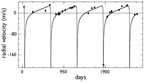
The long-term orbital motion is completely bizarre (as shown by this .mpeg animation) and the corresponding audio file [.wav file here] has a certain demented quality. The signal definitely evolves on longer timescales than shown in this snapshot of the fit:

waveform for hd 128311

Results-oriented planet hunters should definitely be asking, “Does sonification have any scientific utility?”

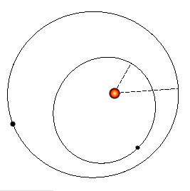
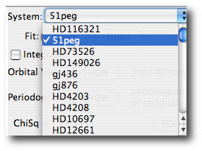
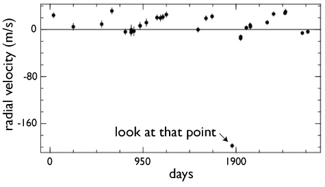
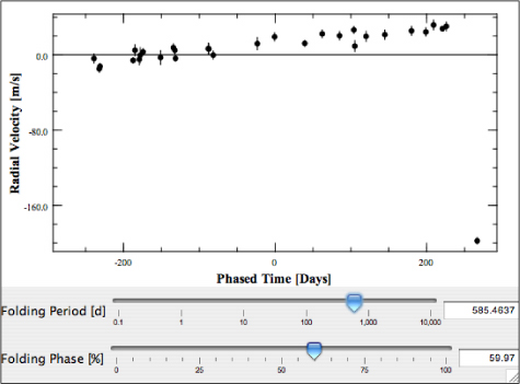
Maybe. I’ll be posting more fairly soon on why we think sonification might be useful, but here’s a straw-man example. Call up the data set for HD 37124 on the console. There are a lot of ways to get an acceptable orbital model for this system, including a panoply of far-out configurations like this one:

hd 37124 alternate orbital configuraton

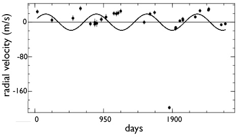
The corresponding waveform looks like this:

hd 37124 alternate orbital fit

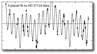
If we sonify the fit, we can literally hear the system going unstable (.wav file here). The question is, can a trained ear “hear” signs of instability well before the actual drama of collisions and ejections occurs?

observations of observations

water glass on a placemat

About two weeks ago, I wrote a post about the Dexter application which is available from the ADS website. Dexter extracts digitized data from image files such as .gifs or .jpgs. We’ve been using it to extract radial velocity data sets for planets that have been published without accompanying radial velocity tables. Our goal is to soon have data sets for all of the planets published to date.

That’ll make oklo.org your site for one-stop shopping.

Eugenio will soon be posting a very interesting discussion of the technique and pitfalls of using Dexter to extract radial velocity data sets. In the meantime, I’ve added a sample dextered data set to the systemic console:

dextered selection for hd50499

The data set HD50499d contains velocities digitized from a figure in the California -Carnegie Planet Search Team’s recent ApJ paper, (entitled Five New Multicomponent Systems). This paper also contains the actual radial velocity data for HD 50499 in tabulated form. This actual data is available on the console by clicking HD50499 (i.e. without the “d” for Dexter).

Try using the console to fit to both the actual data and the Dextered data. You should find that for this particular system, the fits are nearly the same. In this case, Dexter did a very good job of extracting the velocities.

fit to the hd50499 radial velocity data set

The HD 50499 system clearly harbors at least two satellites. One of them has a very long period, considerably longer than 10,000 days. The way to get the console to fit this system is to fix the outer planet period at 10,000 days, while minimizing on the other orbital parameters.

Where we’re at

banana leaf

The systemic collaboration website has now been on the air for six months. Traffic has been increasingly steadily. By the end of April, oklo.org has been averaging 250 visitors a day, with a total of 1661 unique “real” visitors for the month. (This brings to mind a philosophical question: if a tree falls in a forest, and only robots, worms, or replies with special HTTP status codes comment, did it make a sound?)

april showers

The Systemic Team is enthusiastic about a number of improvements that will be coming on line very soon. Here’s a rundown of what to look for during May:

1. Aaron Wolf is putting the finishing touches on the next release of the systemic console. The updated version will have a number of subtle improvements to the existing controls, and will have several completely new features, including a sonification utility and a folding window. Sonification allows the user to create a .wav format audio file of the radial velocity waveform produced by a given configuration of planets orbiting a star:

console sonification controller

As we’ll discuss in future posts, the ability to “listen” to dynamical systems provides a startlingly effective and completely novel way to evaluate the long-term orbital stability of a hypothesized system of planets. For example, when a configuration of planets is stable, one generally gets a sound with a steady timbre: [example 1.5 MB .wav file corresponding to a stable planetary system].

On the other hand, when a configuration of planets is unstable, the radial velocity waveform of the star can get pretty crazy, which can lead to an inifinite variety of very weird sounds: [example 0.5 MB .wav file corresponding to a dynamically unstable planetary system].

2. Stefano Meschiari, who will be transferring as a graduate student to the UCSC graduate program this Fall (yes!), has developed a PHP-based collaborative environment for the systemic project. Think flickr, think myspace, think the Extrasolar Planets Encyclopedia, think seti@home, and think effective scientific collaboration all rolled into one. I’m not kidding, folks, it’s amazing.

Dexter

glasses

Some of the planets that have been detected via the radial velocity technique have been announced in the refereed literature without the supporting evidence of a published table of radial velocities. For the planets that fall in this category, the end-user gets a star name, a list of orbital elements for the planet, and a graph showing a model velocity curve running through the data points. Occasionally, the data is folded, and only a .gif file of the phased radial velocity fit is published.

In a previous post, I wrote about why I can certainly appreciate the planet detection teams’ reasons for not wanting to divulge their radial velocity data when they announce a new planet. If a star has one detectable planet, then the odds are about 50-50 that another planet will be detected after several additional years of monitoring. For a variety of reasons, multiple-planet systems are scientifically more valuable than single-planet systems. In particular, a multiple-planet system (such as GJ 876) tells a fascinating dynamical story, which in turn yields valuable information about the formation and evolution of the planetary system. Obtaining radial velocities is hard, expensive work.

The unavailability of the radial velocity data sets for some of the planet-bearing stars has led to something of a gray market industry in which the radial velocity plots of the parent stars of interesting multiple-planet systems such as HD 82943 and HD 202206 are digitized, and the radial velocities are reconstructed from the graphs. For an example of this technique, see this preprint on astro-ph.

I bear some of the responsibility for the radial velocity .gif digitization industry. In 2001, a press release was sent out announcing the discovery of eleven new planets. This bumper crop included two particularly amazing systems, HD 80606, and HD 82943. HD 80606 harbors a massive planet on an extremely eccentric orbit, and I was very interested to fit the data myself in order to estimate the uncertainties in the transit windows.

The tabulated radial velocities on which the fits were based were not published, but postscript files showing plots of the radial velocities versus time were posted. I went into the files, and by placing commands to print characters in red, I was able to figure out how the plot was encoded. I was then able to extract the exact measured radial velocities for both HD 80606, and HD 82943 from the press conference postings. I didn’t try to publish the analysis that I did with this data, since the procedure seemed a little under-the-table. I did tell people what I was doing, however, and the radial velocity plots on the websites were soon changed from postscripts to .gif files, which are much harder to reverse-engineer.

One of our initial goals with the systemic collaboration is to provide the ability for anyone who is interested to perform a uniform analysis on all of the radial velocities underlying all of the published planets that make up the current galactic planetary census. In order to do this, we need a mechanism for accurately extracting the data from image files in .gif and .jpg format. Systemic team member Eugenio Rivera has been working on this, and has been getting good results with the Dexter Java Applet (available from ADS). The ADS information page gives the following overview:

Dexter is a tool to extract data from figures on scanned pages from our article service. In order to use it, you need a browser that can execute Java Applets and has that feature enabled. Netscape users can verify this by selecting “Edit” -> “Preferences” -> “Advanced” from the top-bar menu and making sure that the button “Enable Java” is checked.

Dexter can be quite useful in generating data points from published figures containing images, plots, graphs, and histograms, whenever the original datasets used by the authors to produce figures in the papers are not available electronically.

We’ll be posting velocity sets extracted from .gif files shortly, and Eugenio will post a detailed write-up of the technique and pitfalls of “observing” the observations.

Some evidence for the existence of 51 Peg c

This post continues with a thread that we’ve been developing over the past several days (posts 1, 2, and 3). In brief, we’ve found interesting evidence of a second planetary companion to 51 Peg in the published radial velocity data sets.

a single spike in a periodogram

We first used the Systemic Console to recover 51 Peg’s famous (P=4.231 d) companion from the data, and then looked at the power spectrum of the residuals to the single planet fit:

residuals

There is a startlingly large periodicity in the data at a 356.2 day period.

We then used the console to identify this periodicity with an Msin(i)= 0.32 Jupiter-mass planet in an e=0.36, P=357 day orbit.

There’s no question that the addition of this second planet reduces the scatter in the data relative to the model. The question is: can the model be taken seriously? Is 51 Peg “c” really there?

Continue reading

51 Peg c

In the posts for Thursday and Friday, we used the Systemic Console to explore the radial velocity variations of 51 Peg. Aside from harboring the first extrasolar planet discovered in orbit around a Sun-like star, this data set is extraordinary because it contains nearly 270 individual radial velocity measurements taken over a period of over ten years. Very few stars have published data sets that are so extensive.

Get on board!

After extracting the signal of the celebrated 4.231 day planet from the data, we computed a periodogram of the residuals. The calculation shows a strong concentration of power at a 356 day periodicity:

residuals periodogram for 51 Peg

At the end of yesterday’s post, we were left hanging on the suggestion that this strong peak might represent a second planet in the 51 Peg system. Let’s have a look at this hypothesis by making a two planet fit to the data.

If you’ve gone through the systemic tutorials, and are comfortable at the controls of the console, here’s the procedure:

Launch the console and follow the directions given yesterday to obtain the best single-planet fit to the data. Next, activate a second planet, and enter 356. into the data window of the period slider for the second planet. Then, minimize the new planet’s mean anomaly, followed by a minimization on the mass. Next, send all ten orbital parameters for the two planets, along with the velocity offsets off for a polish by the Levenberg-Marquardt algorithm. Note that it’s fine to push the “polish” button several times in succession, to ensure that the algorithm has been given enough iterations to converge to the best fit in the vicinity of your choice of starting conditions.

The console shows that the addition of a second planet improves the fit to the data, dropping the chi-square to 1.7, and reducing the required jitter to 5.4 m/s.

The second planet, which we’ll call 51 Peg “c” (where c stands for “console”, huh, huh) has a period of 356.8 days, a minimum mass of 0.32 jovian masses (slightly larger than Saturn), and an orbital eccentricity, e=0.36. Here’s a link to a screenshot of the console showing all the parameters. This is also an advance look at the next version of the console which Aaron will be releasing in a few weeks.

Using the console’s zooming and scrolling sliders, we can see the modulation of the radial velocity curve. The second planet imparts a visibly non-sinusoidal envelope on the strong carrier signal created by 51 Peg b. The non-sinusoidal shape stems from the significant eccentricity of planet “c”:

radial velocities response from 2 planets

Note that we still have to teach the console to draw smooth curves when the zoom level is high! Look for that improvement to show up in about 2 months or so. There’s a lot of other items ahead of it on the to-do list.

The orbits of the two planets look like this:

51 peg b and c

Does it really exist, this room-temperature Saturn? Is it really out there? Do furious anticyclonic storms spin through its cloud bands? Does it have rings? Does it loom as an enormous white crescent in the deep blue twilight sky of a habitable moon?

Maybe.

Eugenio and I have been working through the weekend to devise statistical tests which can assess the likelihood that this planet exists. We’ll check in shortly with our results

51 Pegged?

Yesterday, we supplied the Systemic Console with the published radial velocity datasets of the the planetary system that started it all, the original gangsta, 51 Peg.

It’s interesting, after more than a decade of observation, to see what happens as a radial velocity time series acquires a long baseline. Launch the Systemic Console, and select 51 Peg from the system menu. You’ll see a plot that looks like this:

radial velocity data sets for 51 Peg

With the “51peg_1.vels” offset slider, it’s easy to separate the two contributing data sets. (One was published by the California-Carnegie Planet Search Team, the other by the Geneva Extrasolar Planet Survey). The Swiss data set gives a long baseline of coverage, whereas the California-Carnegie dataset contains intensive observations taken mostly over the course of a single observing season in 1996. Click on the periodogram, and be patient while the console works through the Lomb-Scargle algorithm. While you’re waiting, you can look eagerly forward to the fact that in Aaron Wolf’s next release of the console (due in a few weeks) the periodogram calculation will be sped up by more than a factor of ten.

power spectrum for 51 Peg

The periodogram has an impressive tower of power at 4.231 days. This dataset contains a whopping-strong sinusoidal signal:

To work up 51 Peg “b”, activate the first row of planetary orbital element sliders and type 4.231 into the period box. Then (1) line-minimize the mean anomaly, (2) line-minimize the mass, (3,4) line-minimize both offset sliders, and (5) line-minimize the period. (6) Activate a small eccentricity, (7) move the longitude of periastron slider off the zero point, and then (8) click the Levenberg-Marquardt boxes to the left of each entry box and polish the fit. (If this sounds like gibberish, yet also exciting, we’ve written three tutorials [here, here, and here] that go into detail regarding the use of the console. In addition, all posts marked “systemic faq” contain information about how to use and work with the console.)

When I do this, the console gives me a single planet fit with P=4.2308 days, M=0.4749 Jupiter Masses, and eccentricity e=0.014. These values are in full agreement with the orbital parameters published in the original discovery paper.

Alert readers are likely grumbling that we’ve made no mention of uncertainties in the orbital elements. This is an extremely important and interesting issue for many systems, and we’ll definitely be posting extensively on the topic and theory of computation of errors in orbital elements of extrasolar planets. The entire Systemic research collaboration, in fact, is primarily concerned with resolving the issue of how to establish confidence levels in various types of planetary system configurations.

In the meantime, however, use the console to compute a periodogram of the velocity residuals to the old-school 1-planet fit. A strong peak stands out at a period of 356.196 days. The chi-square statistic of the 1-planet fit is just over 2.00, and the required stellar jitter is about 7 meters per second. This is significantly higher than the 3-5 meters per second of long-term jitter that is expected for a quiet, old G2 IV star like 51 Peg:

residuals periodogram for 51 Peg

Could there be another planet in the system? Could it be, that the console, by virtue of the fact that it readily combines data sets from different published sources, has found a new world (in a habitable orbit no less)? Tune in tomorrow to find out…

O.G.

Most of the recent scientific papers on the general topic of extrasolar planets start with a sentence very much like this one:

Following the announcement of the planet orbiting 51 Peg (Mayor & Queloz 1995), over 170 planets have been discovered in orbit around solar type stars.

straw

And indeed, Mayor and Queloz’s discovery of the hot Jupiter orbiting 51 Peg was truly a watershed event. Their Nature paper has racked up 764 ADS citations. Of order several billion dollars have been spent (or will shortly be spent) on the worldwide effort to locate and characterize alien solar systems. It’s thus a little weird that the Systemic Console has so far failed to include 51 Peg in its system menu. We’ve just corrected this oversight by adding the two published data sets for 51 Peg.

console selection menu

The closely spaced data near the beginning of the time series is from Marcy et al. (1997), who began intensively monitoring the planet from Lick Observatory as soon as the discovery was announced. The widely spaced data is from the Swiss planet hunting team (Naef et al. 2004), and contains 153 radial velocities obtained over a ~10-year period. The data is catalogued at CDS, and available at this link.

The 51 Peg data sets are interesting for a number of reasons. I’ll check in tomorrow with more details as to why. In the meantime, fire up the console and start finding fits.

systemic 002

There’s a new data set on the Systemic Console. To access it, launch the console, and select systemic002 from the system menu (it’s the second from the bottom of the list).

Let’s just say I’ve often wondered whether these particular data can be modeled by a stable planetary system.

hd 20782 oct 20, 2006 (3.6%)

As advertised in yesterday’s post, three newly published radial velocity data sets have just been added to the system menu of the Systemic Console, and to the www.transitsearch.org candidates list. The data set for HD20782, published by Jones et al. of the Anglo-Australian Planet Search, is definitely the most interesting of the trio. Let’s work the HD 20782 velocities over with the console, and see what they have to say.

sunset

First, fire up the console. (If you use Firefox on Windows, and you’ve had success getting the console to work with that particular line-up, please post a response in answer to Vincent’s comment on yesterday’s post. All of Aaron’s oklo.org Java development has been done on Mac OSX using Safari. Also, we’ve had many reports that the console works well with Internet Explorer on Windows, so if Firefox won’t run the Java, give IE a try. And could someone ask Mr. Bill G. to send me a check for that plug?)

At any rate, the HD 20782 radial velocity data set has one data point that sticks down like a sore thumb:

velocities

Activation of one planet and a little bit of fooling around with circular orbits shows that even when the discrepant point is ignored, the waveform of the planet is not at all sinusoidal. The points contain an almost sawtooth-like progression:

circular orbit fit

Because of the non-sinusoidal nature of the velocities, the periodogram (obtained by clicking the periodogram button) is rather uninformative. There’s a lot of power in a lot of different peaks, and it’s not immediately clear what is going on planet-wise:

periodogram

Aaron has been working very hard on console development, and we will soon release an updated version with a number of absolutely bling features. Ever wondered what your fits sound like? One new feature is a “folding window”, which allows the data to be phased at whatever period one likes. The folding window is very useful for data-sets of the type produced by HD 20782. It quickly reveals that something like a 600 day periodicity brings out the overall shape of the planetary waveform:

folding window

Using 600 days as the basis for a 1-planet fit, activating eccentricity, and using a combination of slider work, 1-d minimization, and Levenberg-Marquardt, eventually produces excellent fits to the data that look like this:

fit to hd20872

Jones et al., for example, in their discovery paper, report an orbital period of P=585.86 days, an eccentricity, e=0.92, a mass (times the sine of the unknown orbital inclination) of Msin(i)=1.8 Jupiter masses, and a longitude of periastron of 147 degrees.

This planet is one bizzare world, and seems to be very similar to HD 80606 b (another oklo.org favorite). The orbital period is 1.6 years. The planet spends most of it’s time out at ~2.6 AU. In our solar system, this distance is out beyond Mars in the inner asteroid belt. Once per orbit, however, HD 20782 b comes swinging in for a steamy encounter with the star. The periastron distance is a scant 0.11 AU, roughly half Mercury’s distance from the Sun. The planet is likely swathed in turbulent white water clouds. Raindrops vaporize as the star looms larger and larger in the sky.

Stars that loom large in alien skies are good news for transitsearch.org, and in the case of HD 20782 b, we here on earth are particularly fortunate. HD 20782 b’s line of apsides lies within about 60 degrees of alignment with the line of sight to the Earth. This raises the a-priori geometric probability of having a transit observable from Earth to a relatively high 3.6%. (The a-priori probability of transit for a planet with a 1.6-year period and a circular orbit is only ~0.3%).

oribital figure