This post continues the oklo.org posts: (1) the black cloud, and (2) disks.

There are two competing, completely distinct theories that describe how a giant planet like Jupiter can be generated from a protostellar disk of gas and dust. The first theory, formation via gravitational instability, lends itself to large-scale hydrodynamical simulations and extraordinary animations that can be downloaded over the Internet. It’s an easy theory to grasp. The second theory, formation via core accretion, presents a more complicated chain of events, but nevertheless contains the story that seems (in my opinionated opinion) to be most nearly correct. Let’s look at what these two theories say, and let’s examine the evidence in favor of and against each.

In the gravitational instability picture, the outer lagging remnants of the molecular cloud core fall in and land on the protostellar disk, causing it to grow in mass. As the disk mass increases, it begins to be influenced by its own gravity. That is, it starts to feel a tendency to fragment in response to its own weight. Simultaneously, the pressure of the gas in each nascent fragment pushes back and partially offsets the fragment’s inclination toward collapse. Pressure thus acts as a small-scale stabilizing influence against collapse. In addition, the differential rotation of the disk (material closer to the star orbits faster) tries to sheer a growing fragment apart. Differential rotation thus acts as a large-scale stabilizing influence against gravitational collapse.

The question boils down to the following: Does gravity win, allowing a Jupiter-mass planet to rapidly form as a condensation in the disk, or do shear and pressure win, keeping the disk free of giant-planet fragments?

The situation lies within the general framework of a linearized hydrodynamical stability analyses, and can be analyzed mathematically. The analysis leads to a so-called stability criterion, the famous Toomre Q:

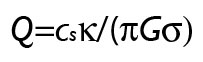
Where c_s is the sound speed in the disk, kappa is the epicyclic frequency, G is Newton’s gravitational constant, and sigma is the disk surface density. If Q<1 at any radius in the disk, then the disk is unstable with respect to m=0 (ringlike) disturbances. If Q is slightly greater than 1, computer simulations show that the disk is prone to strong non-axisymmetric instabilities, and hence experiences exponential growth of disturbances and eventual fragmentation.

As with any seemingly abstruse physical phenomenon, The disk instability analysis can be illuminated with an analogy. In this case, the appropriate analogy involves a rock band, a house party, kegs of free beer, and uninvited punks and thugs.

Neophyte rock bands need to attract audiences for their shows. Hence, they need to provide inducements. Free beer does the trick. Free beer, or more precisely, flyers posted all over a college campus advertising a party serving free beer, act in analogy to the self-gravity of a disk. As I have discovered (through direct experience, back in my reckless, rock-band fronting youth), such a course of action can lead to instability. If you flyer a campus with news of free kegs, then dozens to hundreds of punks and thugs, whom no-one has ever seen before, and whom no-one wants to see again, will descend upon the hapless band’s house-party show. Amplifiers are destroyed. Holes are kicked in sheetrock. The cops show up, and the band does not play. This outcome can be profitably compared to a disk that undergoes a gravitational collapse into Jovian-mass fragments.

[Above: Our bass player (at a show of ours that was shut down by the cops after several songs). He later graduated with a Ph.D. in Physics, after defending his dissertation on 2D quantum black holes.]

In practice, however, the police do not always show up at house-party shows. Sometimes, the band gets to play. This happier outcome is abetted by two stabilizing effects. Just as in the case of the disk gravitational instability, one of these stabilizing effects operates on large scales, and the other operates on small scales. On the large scale, one can create an analog of “differential rotation” with a lack of specificity on the flyers regarding the precise time of the show. Punks drift in. They see that they don’t particularly like how the band sounds. They see the long lines to the kegs. They drift away. The band plays its entire set to a modest audience, and the cops don’t show up. Support on small scales, the analog of “pressure” is provided by a quite different effect: body odor. The thugs that show up invariably smell poorly, and the unpleasantness associated with a sweaty throng of them will drive some away. If the pressure is high enough, that is, if the thugs smell badly enough, then the show proceeds, and instability is again averted.

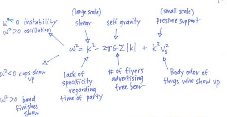
For readers familiar with the linearized analysis that leads to the Toomre Q criterion, here’s an illustration of how the analogy can be applied to the standard WKB dispersion relation:

In a future post in this series, we’ll explain why the weight of observational and theoretical evidence seems to be shifting against the gravitational instability hypothesis. The computer simulations, which become ever more impressive with each inexorable tick of Moore’s law, show that in order for fragments to form and then last as planets, the rate of cooling in the disk must be extremely efficient. Rapid cooling robs a nascent fragment of its ability to produce pressure, and hence permits gravitational collapse. Perhaps more importantly, the computer simulations also show that a disk will suffer from a whole panoply of instabilities before its mass grows large enough to trigger the full-blown collapse of Jupiter-like planets.

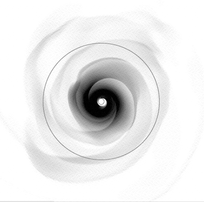
These instabilities take the form of spiral waves of the same type that occur in spiral disk galaxies such as M51, shown in the HST photo at the top of the post. In a protostellar disk, the spiral wave action pushes pulse after pulse of gas out of the regions of the disk that are in the most danger of fragmenting directly into planets. Some of this gas is forced to large distances from the central star, while the majority flows inward and eventually winds up on the star. In all likelihood, most protoplanetary disks manage to avoid direct fragmentation.

Frequent visitors to oklo.org will have noticed that the new posts have dried up over the past several days. I was out of town to attend the 2nd annual Mitchell Institute Symposium at Texas A&M. This is a conference that brings together speakers from a broad range of sub-disciplines in Astronomy and Physics. Ten gallon hats off to Texas! I had a great time. Warm weather, informative talks, and the Aggies all called me “Sir”. My plan for next week is to get the UCSC Banana Slugs to start up with that tradition.

As part of the conference, I was asked to give a public talk on Extrasolar Planets. It was an all-day scramble on the laptop to get all my slides together into a coherent whole, but the talk ended up being a lot of fun. The audience was highly informed and engaged. The TAMU Physics Department definitely got the word out. I was completely stunned this morning to find that I was on the the front page of the Bryan-College Station Eagle, and I was even recognized at the College Station Airport cafe while I was waiting for my flight out. Unbelievable.

Here’s a link to a quick-time movie, as well as a .pdf file with the slides that I showed during the talk. I’ve also put the sound files (you had to be there to know what I’m talking about) here, here, and here in .wav format. A future oklo post will go into much more detail about what’s being heard in these files, and how they are generated.

If you’re new to the site, here’s a bit of information. Oklo.org is the home base for the systemic collaboration, which is a public participation research project aimed at obtaining a better characterization and understanding of extrasolar planets. Everyone is invited to participate, and details and updates are given regularly in our systemic faq posts.

We have been developing both the oklo.org site, as well as the systemic console using a Mac OS-X platform. We have been testing both the site and the console using Internet Explorer, and we have gotten generally good results, but it is clear that some users are experiencing problems. We are working hard to clear these issues up. We’re astronomers by trade, and, and sadly, at the moment, it’s strictly amateur hour when it comes to website development. As an example, you should see a menu of links directly to your right. I recently saw the oklo.org site on a Windows-IE combination in which the links had been mysteriously pushed all the way down to the bottom of the page. I had to scroll all the way down to even see them.

Also, if you are a Macintosh user, run the console in Safari. There is a still a Java issue with the Firefox on OS X. Firefox should, however, work fine on both Linux and Windows machines if your Java libraries are up to date…

In early June of 2001, I was sitting at my desk at the NASA Ames Research Center trying to debug a computer simulation. Outside my window, the traffic was gridlocked on Highway 101. The distant folds of the Diablo Range shimmered in the California Sun. The phone rang, jarring me out of my abstracted state of mind.

“Dr. Laughlin? Its Robin McKie of the London Observer.”

His voice seemed friendly and reasonable, and I’ll admit that I was pleased to have warranted a call from an overseas reporter. To the best of my recollection, our conversation started something like this:

“Well the reason I’m calling is because I recently saw an abstract of your work concerning this so-called idea of `Astronomical Engineering’, and I was wondering if you could take a few minutes to fill me in on what its all about?’’

Continue reading →

One evening last August (0. 12. 19. 12. 10. 10.) I was filling my car with gasoline. Venus hung low and bright above the horizon in the deep blue twilight. In the foreground stood the glowing red and yellow symbol of Shell Oil. Swirling coils of aromatic hydrocarbons dissipated in the cool marine air.

The ancient Maya were obsessed with Venus. At the times when it was visible, they covered windows and doorways to protect against its rays of mirrored sunlight.

Venus’ brilliance in our skies arises partly because of its proximity, and partly because it is completely covered with thick white clouds that drift through the upper layers of a CO2 atmosphere roughly 100 times more massive than Earth’s. Venus, however, may not always have been so inhospitable. The high Deuterium to Hydrogen ratio in its atmosphere indicates that it has lost a lot of water. It is possible that during the first billion years of the Solar System’s history, Venus had liquid water, perhaps even an ocean, on its surface. If this was the case, then Venus shone down with less brilliant menace in the Archean skies.

In two, or perhaps three billion years from now, the Earth will have shared Venus’ fate, and will glow with pure-white intensity in the salmon twilight of the Martian evenings.

(Note: the above image of Venus in transit is a screenshot detail from a .jpg image on the website of the Venezuelan Centro de Investigaciones de Astronomia.)