We’ve noticed that fresh content encourages regular return visits to oklo.org.

With that sentiment in mind, here’s a stop-action .mpeg4 animation of the newly discovered 2:1 resonant planetary system orbiting HD73526. The planets are represented by red and green peppercorns, and a kumquat stands in for the central star:

hd73526.mov

If the version above won’t load in your browser, try this one. Rest assured that the systemic team is hard at work on more substantive posts (including some very interesting new exoplanet-related results), so check back frequently!

It’s been unseasonably cold in Santa Cruz. Last night, a freak hailstorm left drifts of icy planetesimals lodged between the leaves of the banana tree outside the bedroom window.

My office, however, is nice and warm. This is because two 2.5 Ghz G5 processors are running mercury.f at full tilt to simulate the formation of habitable planets orbiting low-mass red dwarf stars. The calculations are being done in preparation for Ryan Montgomery’s presentation at AbSciCon in Washington D.C. Two weeks to go.

Two Spheres Within A Sphere Alexander Calder, 1931

Most of the runs have already been carried out using a linux-based beowulf cluster, which is able to run more than 100 individual simulations at once. Each of these simulations starts with 1000 low-mass planetesimals, and calculates the final stages of terrestrial planet formation by allowing the orbiting planetesimals to interact under their mutual gravitational influence. Collisions and ejections gradually winnow the initial swarm down to a few surviving terrestrial mass planets. By doing many simulations, we build up a statistical picture of what the distribution of red dwarf planetary systems should look like.

The desktop computer contains the fastest individual processors to which we have full access. We’ve therefore harnessed it for a single test-case run to investigate the overall sensitivity of our results to the number of initial particles. The processors have spent the last six weeks evolving a system that had an initial distribution of 10,000 small planetesimals. At the projected rate of evolution, it should just manage to finish up just in time. Indeed, if you see Ryan hunched over his laptop at the conference, you’ll know what he’s up to.

John Chambers’ Mercury code (like the Systemic Console in integrator mode) is based on the method of direct summation. At each timestep, each particle in the simulation experiences a gravitational attraction of the form GM/r^2 from every other body in the system. For a 10,000 particle system, that means of order ((10,000)x(9,999))/2=49,995,000 square roots must be computed every timestep (and the actual number is higher, because each timestep consists of a considerable number of substeps). As the number of particles increases, the cost of the calculation increases as the number of particles squared. Our 10,000 particle simulation is 100 times more expensive than the 1,000 particle production runs, and thus pushes the limits of what we can currently readily do.

Many problems in gravitational N-body dynamics can be solved without resorting to direct summation. In essence, this is because to a high degree of approximation, the gravitational attraction from distant particles depends only on the the rough location and total mass of the distant particles. One gets nearly the same result by lumping distant particles into a single, equivalent, large-mass particle:

Using clever variations of this basic idea, one can speed up an N-body (or equivalently, an SPH) calculation enormously. Competitive N-body codes for large-N problems, such as the collisions of galaxies or the formation of structure in the early universe, generally scale as N log(N). For large N, the difference between N^2 and N log(N) is profound. With a million particles, for example, an N log(N) calculation is a cool 72,382 times faster than the brute-force N^2 approach.

One might ask, is there a way to further speed up the computation of the gravitational forces so that finding the accelerations becomes an order N process?

Remarkably, an order-N computational N-body method was employed by Erik Holmberg of the Lund Observatory in Sweden in 1941. Instead of integrating the equations of motion with a computer, Holmberg modeled a two-dimensional system of gravitating particles as an actual physical distribution of movable light bulbs laid out on a gridded sheet of dark paper! Because the intensity of light from a point source diminishes as 1/r^2, one can directly relate the intensity of the light at a particular spot to the gravitational acceleration. The order-N^2 process of computing the gravitational force on a given particle from all of the other particles reduces to a measurement of the total intensity of light in two perpendicular directions using a photocell and a galvanometer. Since one set of measurements is required for the location of each light bulb, the method scales as N. Here is a link to Holmberg’s paper. It’s one of my all-time favorites.

With his analog method for computing the net gravitational acceleration on each of his light bulb “point masses”, Holmberg could compute the change in trajectories which would occur over a time interval using a simple integration scheme such as Euler’s method. A timestep would then be completed by moving all of the light bulbs to their updated positions, at which point a new estimate of the gravitational acceleration could be made. Holmberg’s scheme allowed him to gain a better understanding of important aspects of the dynamics of close encounters between disk galaxies, including the phenomena of orbital decay and the formation of tidal tails:

There is an interesting lesson to be drawn. Use of an analog method reduces an N^2 direct summation computation to order N, foreshadowing a time when quantum computation will similarly reduce the computational time for direct summation from N^2 to N. Until that time, however, the light-bulb method beats all others as the number of particles approaches an arbitrarily large value.

In honor of analog methods, here’s a home-made mpeg-4 stop-action animation of a peppercorn orbiting a kumquat in an ellipse with e=0.90. (Try this version if the other one loads a screen of gibberish).

.

The black cloud post describes how the formation of a star and a planetary system can be traced back to the moment when a dense core within a giant molecular cloud begins to suffer an inside-out collapse. The gas at the center of the cloud collapses first, and congregates into the beginnings of a hydrostatically supported protostar. The overlying regions thus lose their support and begin to career inward as well. A wave of collapse radiates outward from the center of the cloud, triggering a downward avalanche of gas and dust. Computer simulations show how gas that has fallen from large distances comes together to form a protostellar disk in orbit around the nascent central protostar. In the image shown below, a simulation of the earliest phases of our own solar system show a region (viewed edge-on) that is several hundred astronomical units across, and plotted 40,000 years after the collapse has started. At this stage of the simulation, roughly half of a solar mass of material has collected in the central protostar, and another half a solar mass or so is orbiting in a very massive protostellar disk.

As the disk grows in mass, it begins to feel its own self-gravity, and some regions begin to collapse under their own weight. At the same time, the pressure of the gas in the disk resists the tendancy to collapse, and the differential rotation of the disk acts to sheer out fragments as they grow. This process can also be simulated, and the result is spiral waves (viewed here from above):

The presence of the spiral waves causes angular momentum to be transferred outward through the disk, while allowing the majority of the mass to flow inward to eventually join with the central protostar. Even after the spiral waves have dissipated, there must exist continuing source(s) of angular momentum transfer through the disk. The identification of these mechanisms is still an active area of research. Possible mechanisms that might operate after the disk is no longer massive enough to support self-gravitating spiral waves include the magneto-rotational instability, as well as convection-driven turbulence in the disk. One way or another, angular momentum transport was extremely effective. The initial cloud that formed our solar system was rotating more or less uniformly, wheras at the present day, there is nearly a complete separation between mass and angular momentum in the solar system. The Sun contains more than 99.8% of the mass, and the planets carry more than 98% of the system angular momentum.

When I give public talks on planet formation, I like to show the above image (taken by HST, and released in 1995) of a protostellar disk, or proplyd, in the Orion star-forming region. We see the cold proplyd from an edge-on vantage, against a diffuse background of hot glowing gas. This disk is at a somewhat later phase of evolution than the ones pictured in the above simulations. It’s roughly 1400 AU across, which is more than 15 times the diameter of Neptune’s orbit, and considerably larger even than the orbits of the newly discovered Kuiper belt objects 2003 UB313, and Sedna. To give an idea of scale, I’ve integrated both Sedna and 2003 UB313 for one Sedna orbit (12,050 years) and plotted their positions relative to the plane of our solar system and superimposed (to scale) on the proplyd. Sedna, is currently in the portion of its orbit where it is speeding (in its rather lazy, loosely bound fashion) through perihelion, and hence the dots plotted at 120.5 year intervals in that region are spaced widely apart. Seen from above, Sedna’s eccentric (e=0.855) orbit would have a aphelion point considerably beyond the radial edge of the proplyd.

Continue reading →

Frequent visitors to oklo.org will have noticed a definite fall-off in the number of recent posts. This was a direct result of the start of the winter quarter here at UCSC, but now things are rolling, and the systemic team is working hard to prepare the next phase of the collaboration.

Last week was also the 207th meeting of the American Astronomical Association. I took a one-day trip to Washington in order to give a talk at Tuesday’s extrasolar planets session entitled, “From Hot Jupiters to Hot Earths“. I teach class on both Monday and Wednesday mornings, so the trip was more of a lightning raid.

I arrived at Dulles Airport at 6 am, after an overnight flight. My talk wasn’t finished, so I sat in an empty departure lounge for several hours and worked on the slides. By mid-morning, I realized that I had better head to the venue. I took a cab to the conference hotel, tapping on the laptop for most of the way.

Hundreds of astronomers were thronging in the hallways. I studied the posters that had been set up in a large exhibition hall, and then went to hear NASA Administrator Griffin give a keynote address, the gist of which was clearer than this snapshot (taken under low-light conditions).

Two of the things he said stuck in my mind.

Like it or not, NASA has been charged to fly to the moon for reasons that are completely divorced from astronomy, and this means that there will be opportunities to use a lunar platform for observations of extrasolar planets. Transit photometry of nearby stars, especially M-type stars, jumped to mind, but clearly, there is a serious opportunity right now to start thinking outside the box.

He also said that the primary education and outreach mission of NASA should be to inspire by doing “cool things”. I do remember watching the last Saturn V’s blast off for a lunar destination, and I remember, a few years later, learning in grade school science class, about the Space Shuttle, that “pickup truck into orbit”, and feeling distinctly less inspired. In the intervening years, my list of the coolest NASA things runs along the lines of, Voyager, HST, WMAP, Cassini-Huygens, and Spitzer. And there’s also the BPP project. (For more detail on interstellar missions, Paul Gilster’s Centauri Dreams is always the place to go).

Uh, my talk wasn’t all it could have been. In order to facilitate rapid transitions between the session speakers, everyone’s slides were uploaded to a central server. The server was running Windows, and all the Powerpoint presentations looked exactly like they were supposed to. Full screen ahead. As a Keynote user, however, my slides were in the form of .pdfs. They looked just fine in the speaker ready room, but then, when I stepped up to the podium, I was aghast to see that my .pdfs were displaying on only on a small portion of a screen containing an acrobat viewer, complete with a sneak “preview” and a sneak “review” of the next and previous slides. The resolution was too low to see any detail. Score one for Mr. Bill Gates.

For the record, though, here are the slides (full resolution .pdfs).

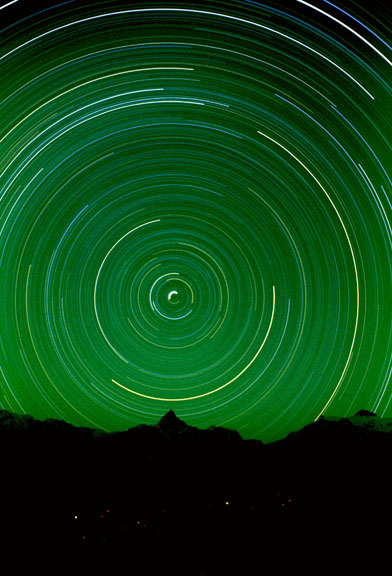
Let a pebble slip from your hand and it falls straight to the ground. Toss the pebble sideways, and it traces a parabolic arc through the air. Imagine throwing the pebble sideways with even more speed. It lands further away. Imagine throwing the pebble with such great velocity that the surface of the Earth begins to curve away beneath it as it falls. In the absence of air friction, a pebble thrown sideways with sufficient velocity will fall in such a way that the Earth curves continuously out from underneath. The pebble falls endlessly without ever touching the ground. It is in orbit.

The idea that an orbit is the state of a body in continual free-fall can be traced to the 1600s, and was first stated in print by Robert Hooke, whose paper entitled, “The Inflection of a Direct Motion into a Curve by a Supervening Attractive Principle” was read to the Royal Society on May 23rd 1666. Robert Hooke’s fame and reputation have spent the last three hundred and twenty years in Newton’s shadow, but he was a tremendously inventive scientist, and indeed, was one of the founders of what we now consider the scientific method. (See, for example, the recent Hooke biography, “The Forgotten Genius” by Stephen Inwood). Hooke, drawing on the earlier ideas of William Gilbert and Jeremiah Horrocks, and profiting from conversations with fellow Royal Society member Christopher Wren, realized that if the Sun exerts an attractive force on bodies in space, then “all the phenomena of the planets seem possible to be explained by the common principle of mechanic motions.” Hooke had an intuitive (but non-mathematical) understanding of the the orbit in the sense described in the paragraph that opens this post.

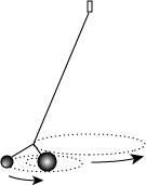
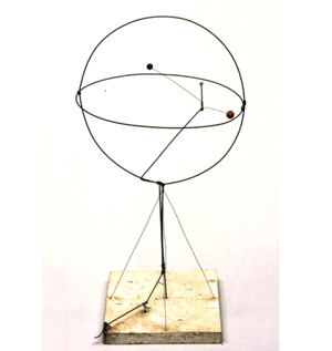
Robert Hooke was shouldered with a bewildering variety of interests and responsibilities. One of his many jobs was to produce weekly demonstrations for the entertainment and edification of the Royal Society. In order to illustrate his concept of the planetary orbit, he devised a demonstration that provided a suggestive analogy. A bob was placed on a long string pendulum. Tension from the string provided a central attractive force, and a sideways push provided the requisite tangential motion. When given a sideways push of exactly the correct speed, the bob would swing in a circle. When started at other speeds, it traced an elliptical path. With this simple device, Hooke was able to illustrate how an orbit is a compound of tangential motion and an attractive radial force.

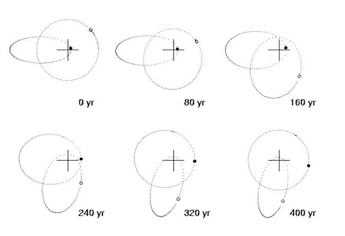
Hooke then made the analogy more elaborate by attaching two bobs to the end of the string. Once set in motion, the two bobs would orbit each other, while their center of mass orbited the center of attraction:

In 1670 , Hooke delivered a Cutler lecture at Gresham College, entitled, “An Attempt to Prove the Motion of the Earth by Observations”. The written version of this lecture contains three remarkable postulates, including, (1) a specification of the concept of universal gravitational attraction, that is, that mass attracts mass, (2) the assertion that all bodies “that are put into a direct and simple motion would continue to move in a straight line unless deflected”, and (3) the hypothesis that the attractive gravitational force falls off with distance. Taken together, these ideas are a remarkably correct qualitative formulation of the foundations of gravitational dynamics. Had Hooke been equipped with the mathematical skill to express his three ideas quantitatively, he would have gone very far indeed.

At the same time that Hooke was demonstrating his pendulum analogy to the Royal Society, Isaac Newton was nearing the close of his Anni Mirabiles. By 1666, Newton, who was working in total isolation, had found a quantitative model that explained the circular orbit, and also showed that gravity is manifested by an inverse square law of attraction.

I began to think of gravity extending to the orb of the Moon, & (having found out how to estimate the force with which a globe revolving within a sphere presses the surface of the sphere) from Kepler’s rule of the periodical times of the Planets being in sequialterate proportion of their distances from the center of their Orbs, I deduced that the forces which keep the Planets in their Orbs must [be] reciprocally as the squarres of their distances from the centers about which they revolve: & thereby compared the force requisite to keep the Moon in her Orb with the force of gravity at the surface of the earth, & found them to answer pretty nearly. (All of my Newton quotes are drawn from Richard Westfall’s “Never at Rest — A Biography of Isaac Newton“)

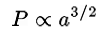
Here’s what Newton is saying. Kepler’s Third Law holds that the orbital period of a planet is proportional to the semi-major axis of its orbit to the 3/2 power, that is,

For the simplified case of a satellite in a circular orbit, the semi-major axis, a, is just the orbital radius, i.e. a=r. In Newton’s state of understanding in 1666, the “centrifugal” outward force an orbiting satellite must cancel the inward force exerted by gravitational attraction from the central body. The gravitational attraction is assumed to be spherically symmetric and to fall of with some power of the distance. That is,

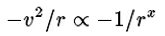
where x needs to be determined. The fact that distance is rate multiplied by time implies that

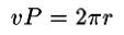
and therefore

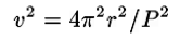
This means that

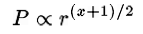
and if Kepler’s third law is to be satisfied, then x=2. Newton had realized that Kepler’s third law implies that gravity is an inverse-square force.

Newton had thus found a workable mathematical model for the circular orbit in 1666, but at that time, he was behind Hooke in terms of his intuitive understanding of the actual physical situation. Newton’s initial conception of the orbit was one of a mechanical equilibrium, in which an innate tendency to recede during circular motion is balanced by a gravitational attraction. In reality, Hooke’s concept of the orbit as the state of continual free-fall, a state of disequilibrium, is the correct notion.

On Nov. 24, 1679, Hooke, in his capacity as the secretary of the Royal Society, wrote a letter to Newton in order to solicit a discussion of orbital dynamics. Hooke was likely quite proud of his theories concerning orbital motion, and he may well have been eager to bring his ideas to Newton’s attention.

Let me know your thoughts of that of compounding the celestaill motions of the planets of a direct motion by the tangent and an attractive motion towards the centrall body.

Hooke had no way of knowing that Newton had already thought carefully about orbits. It is likely that as soon as Newton saw Hooke’s phrase, he immediately saw that it represented an improved qualitative conception of orbital motion. He quickly wrote back to Hooke, and politely declined the offer of an extended dialog. He, was, he said, too busy with other studies.

And having thus shook hands with Philosophy, & being also at present taken of with other business, I hope it will not be interpreted out of any unkindness to you or the R. Society that I am backward in engaging my self in these matters…

Nevertheless, the correspondence between the two continued through several more letters. By January 1680, Hooke had managed to guess (on the basis of two incorrect arguments that combine by chance to give a correct formula) that the gravitational force obeys an inverse square law. What he could not prove, however, was what the general path of an orbiting planet is an ellipse (that is, he could not go beyond the special case of the circular orbit). The fact that the planetary orbits have elliptical figures was then known empirically from Kepler’s First Law, which states that planetary orbits are ellipses with the Sun at one focus.

On January 6th, 1680, Hooke took the liberty of informing Newton of the inverse square law, “My supposition is that the Attraction always is in a duplicate proportion to the Distance from the Center Reciprocall…”, and in a letter on the 17th of January, he further urged Newton to find the general mathematical description of a planetary orbit,

I doubt not but that by your excellent method you will easily find out what that Curve must be, and its proprietys, and suggest a physicall Reason of this proportion.

Hooke’s letters of November through January of 1679-80 seem to have greatly annoyed Newton. With his formidable intuition and dismal mathematical skills, Hooke was steadily blundering toward the pedestal where he could claim the renown of explaining the “System of the World”. Without informing Hooke, Newton carried out (in early 1680) a marvelous derivation that showed that the path of a planet is an ellipse, and simultaneously proved Kepler’s Second Law, which states that the radius vector of a planet sweeps out equal areas in equal times, and which is a statement of the principle of the conservation of angular momentum.

Years later, soon after the appearance of the Principia, when Hooke claimed that Newton had plagiarized his ideas, Newton lashed out at Hooke in a letter to Edmund Halley:

Should a man who thinks himself knowing, & loves to shew it in correcting & instructing others, come to you when you are busy, & notwithstanding your excuse, press discourses upon you & through his own mistakes correct you & multiply discourses & then make use of it, to boast that he taught you all he spake and oblige you to acknoledge it & cry out injury and injustice if you do not, I beleive you would think him a man of a strange unsociable temper.

Robert Hooke, that man of strange unsociable temper, is nevertheless a man after my own heart. Newton is so far out on the curve that I can’t relate to him at all. I have no concept of how his mind operated, but Hooke, Hooke would be a fantastic person to have a beer with. I can appreciate the way he thought by analogy. I greatly admire his demonstrations, even if they aren’t fully rigorously correct.

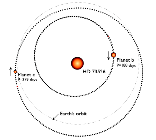
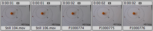
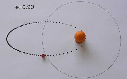
With Hooke’s approach in mind, let’s look at some elliptical orbits. When an ellipse has zero eccentricity, the two foci come together, and the ellipse is a circle. A planet on a circular orbit travels at constant speed, and its positions at a hundred equally spaced time intervals are equally spaced:

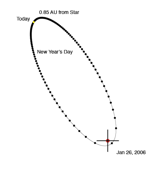
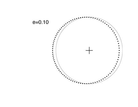
When the eccentricity reaches 0.1, the orbit looks very much like a shifted circle. When the planet is closest to the Sun (the point known as perihelion), it is moving faster. If you look carefully, you can see that the dots are spaced just a bit more sparsely on the right side than on the left. The e=0.1 orbit just below is very similar to the orbit of Mars, which has an eccentricity e=0.0935. In all of the following figures, the e=0 circular orbit is also shown for comparison:

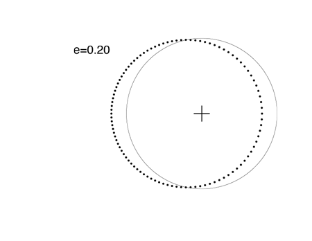
Among the eight major planets in our Solar System, Mercury, with e=0.205, has the most eccentric figure. Mercury’s orbit is almost identical to the orbit in this plot, which has e=0.20:

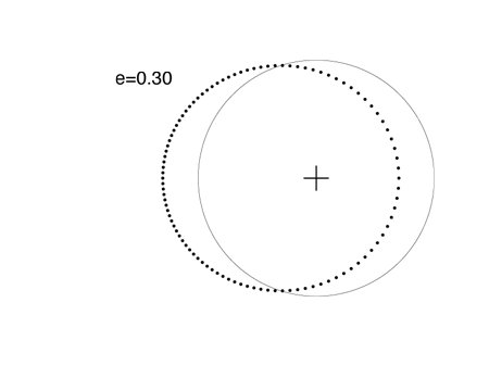
Planets “c” and “d” of the Upsilon Andromedae system have eccentricities of e=0.27 and e=0.28 respectively. Their orbital figures are quite close to this orbit, which has e=0.3:

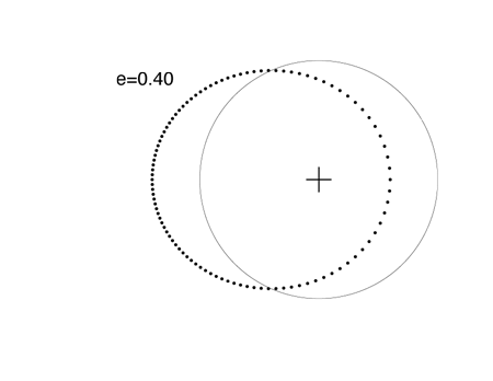
70 Vir b was one of the first extrasolar planets to be discovered. It has a very well defined orbit with e=0.4:

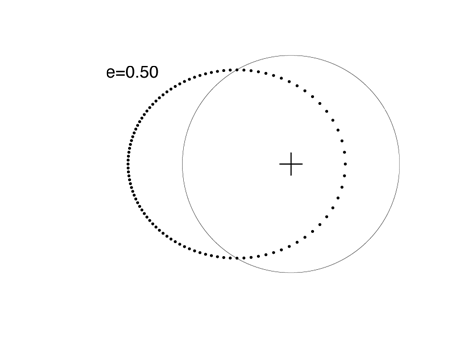
When e=0.5, it’s impossible to mistake the ellipse for an off-center circle. The extrasolar planet GJ 3021 b has an eccentricity e=0.511, which is close to e=0.5:

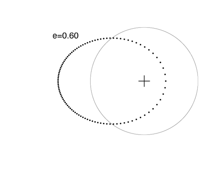
At an eccentricity e=0.6, the brevity of the periastron swing is highly pronounced:

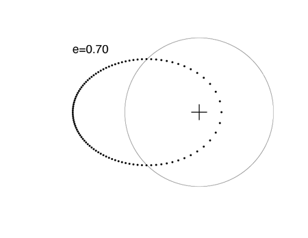
When e=0.7, the planet is 5.667 times closer to the star at periastron than at apastron.

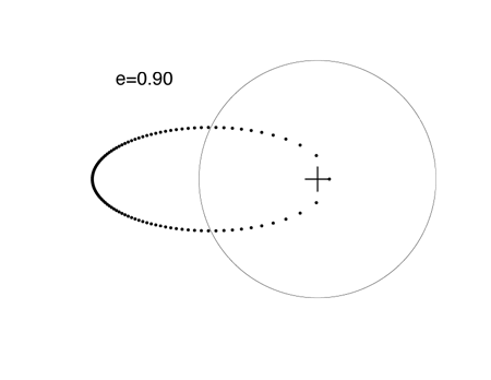
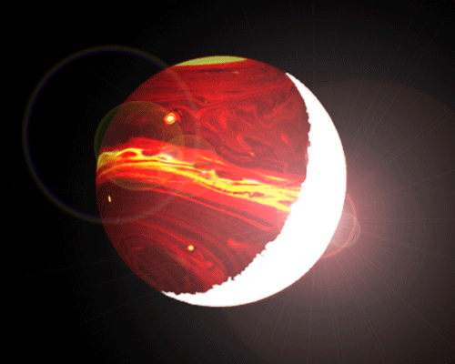
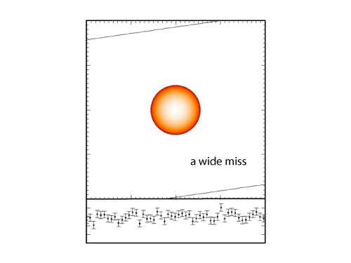
The extrasolar planet with the highest known eccentricity, HD 80606 b, has an 111 day orbital period and e=.938. See my article on this strange world posted last month. Because it dives in so close to its parent star, HD 80606 b is an interesting transit candidate, but a transitsearch.org campaign carried out last year did not detect transits. We’ll try again this year during the upcoming transit opportunities.

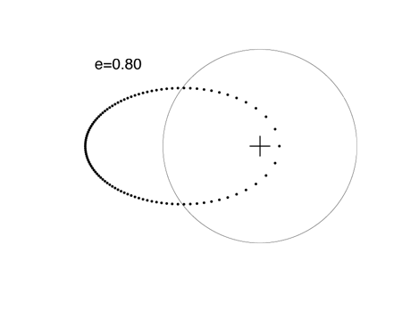
Do you give talks on extrasolar planets? High-resolution .pdf files of the above orbital plots are free here for the taking: e=0.0, e=0.10, e=0.20, e=0.30, e=0.40, e=0.50, e=0.60, e=0.70, e=0.80, e=0.90.

On Dec. 12, 2005, we arrived at Kansai with the Sun low on the horizon, casting orange shafts through the plane. Whitecaps were frothing on the Inland Sea. The airport is built on two 4 kilometer by 1 kilometer artificial islands, and is connected to Honshu by a 3 kilometer bridge that cost 100 billion yen. Beneath the vast new terminal, an attendant with a pressed shirt and tie helped us navigate the ticket machines to buy two Haruka Ltd. express tickets to Kyoto. The bullet train pulled away as soon as we stepped on, gliding glass-smooth through the night blur of an endless city.

That night, in a room in the hyper-modern Hotel Granvia, I lay awake, jet lagged and alert, listening to the faint rush of warm air flowing from a network of unseen ducts. Outside, the lights of the city were a panoply of mysterious characters and sparkling complexity, illuminating blocks of buildings that stretched away in all directions to the dark mountainous horizon. I was suddenly brought around to a simple fact that I always find startling:

No one arrived from outer space to build all this. In a very real sense, the planet Earth has done has done all this itself.

Continue reading →

A hundred, or even fifty-five years ago, it was thought that Mars and Venus might both harbor complex life, and the aspirations of science fiction writers and adventurers were pinned squarely on those two worlds. With the advent of space probes, however, we visited these planets, and the dream of lush sister worlds orbiting our own Sun was shattered. Mariner 2 reported the hot sulfurous truth about Venus; the crushingly poisonous atmosphere has no water and is hot enough to melt lead. Mars, when brought into focus by the Mariner and Viking probes, was only somewhat less disappointing. Aside from flood channels that have been bone-dry for billions of years, and the faint possibility that microbial life clings to the fringes of hypothesized hot springs, Mars has little to offer in the way of luxurious alien romance. For this, we must turn to other planets around other stars.

But we can still speculate. What would have happened if our solar system harbored a second, truly Earthlike, truly habitable world? What if there had been a genuine marquee destination for the cold war rockets?

Is such a planetary configuration dynamically feasible? We know that the continuously habitable zone around a star like the Sun may be relatively narrow. Is it possible to fit two Earth-mass planets within? More specifically, what would happen if we placed an exact copy of the Earth in the Earth’s orbit, with Earth’s orbital elements, and with the only difference being a 180 degree advance in the mean anomaly. In other words, what would the dynamical consequences be if Earth had a twin on the other side of the Sun?

In 1906, the German astronomer Maximillian Franz Joseph Cornelius Wolf discovered an asteroid at roughly Jupiter’s distance from the Sun which was orbiting roughly 60 degrees ahead of Jupiter, and thus forming a point of an Equilateral triangle with Jupiter and the Sun. It was soon realized that the orbit of this asteroid was very stable, since it is positioned at the so-called Jovian L4 point, one of the five stable Lagrangian points associated with the Sun and Jupiter. These points represent special solutions to the notorious three-body problem, and were discovered in 1772 by the Italian-French mathematician Joseph Louis Lagrange. The following diagram was lifted from the wikipedia:

Wolf named his Jupiter-L4 asteroid 588 Achilles, after the sulky Greek hero of Homer’s Illiad. A year later, August Kopff discovered a similar asteroid, this one orbiting at the so-called L5 point, 60 degrees behind Jupiter. In keeping with the Homeric tradition launched by Wolf, Kopff named his asteroid 617 Patroclus, after Achilles’ gentleman friend and fellow greek warrior. Thus, with fitting cosmic symmetry, the two heroes were immortalized in the heavens to either side of mighty Jupiter.

Later in 1907, Kopff discovered a third co-orbital asteroid of Jupiter, this one near L4, which he named 624 Hektor, in honor of Achilles’ Trojan nemesis. Hubble Space Telescope observations indicate that Hektor is actually a contact binary,
in which two asteroids are effectively glued together by their weak gravity. In 1908, Wolf discovered yet another object (659 Nestor) near Jupiter’s L4 point. It was clear that a whole class of Trojan asteroids existed, and in order to keep things straight, it was decided that asteroids found near L4 would be named after Greeks (the Greek camp), whereas asteroids near L5 would be named after Trojans (the Trojan camp). Hektor and Patrocles, who were thus orbiting in the camps of their respective enemies, were given the unique status of spies.
Nearly two thousand trojan asteroids are now known. Even minor figures such as Hektor’s infant son (1871 Astyanax) are now attached to asteroids, and the Illiad’s roster is nearly completely exhausted. Trojan asteroids of recent province, such as 84709 2002 VW120 are relegated to the status of neutral observers.

The US Navy maintains a website that charts the orbital motion of a number of trojan asteroids. (The Navy’s involvement seems rather appropriate, as it was Helen, whose beauty was sufficient to launch a thousand ships, who touched off the Trojan War.) As a Trojan asteroid orbits the Sun, it also orbits about its Lagrange point by executing two essentially independent librations. The combination of the two librational motions leads to an intricate motion when viewed in a frame that rotates along with Jupiter.

Back to our hypothetical Doppelganger of the Earth.

In the language of Lagrange, when we place a new world on the opposite side of the Sun from the Earth, we have populated the L3 point. A linear perturbation analysis shows that if an object at L3 is perturbed, then the orbit will drift steadily away from the initial L3 location. That is, the orbit is linearly unstable, in contrast to the the orbits at L4 and L5, which are linearly stable, and hence stick around in the vicinity of trojan points, even when they are subjected to orbital perturbations.

A computer is required to find out what would happen to the orbits of the Earth and our hypothetical twin planet. It turns out that the motion is nonlinearly stable. The Earth and its twin would be perfectly content, and, in a frame rotating with a 365 day period, the motion of the two planets over a period of years would look like this:

As one planet tries to pass the other one up, it receives a forward gravitational pull. This forward pull gives the planet energy, which causes it to move to a larger-radius orbit, which causes its orbital period to increase, which causes it to begin to lag behind. Likewise, the planet which is about to be passed up receives a backward gravitational pull. This backward pull drains energy from the orbit, causes the semi-major axis to decrease, and causes the period to get shorter. The two planets are thus able to toss a bit of their joint orbital energy back and forth like a hot potato, and orbit in a perfectly stable variety of a 1:1 orbital resonance, known as a horseshoe configuration. The horseshoe orbit is an example of the negative heat capacity of self-gravitating systems, which is one of the most important concepts in astrophysics: If you try to drain heat away from a self gravitating object, it gets hotter.

Here’s a thought. It is dynamically possible that 51 Peg b (or any of the other extrasolar planets that do not transit within the predicted window) is actually two planets participating in a stable 1:1 orbital resonance…

While we’re on the topic of far-out planetary configurations, another type of allowed 1:1 configuration is the 1:1 eccentric resonance, an example of which is shown below. In this situation, two Jupiter-mass planets share the same period, but have very different eccentricities.

Over time, the planets pass their eccentricity back and forth in an endless resonant cycle. If one of these configurations is found orbiting a sun-like star, it will induce a very distinctive radial velocity curve which will allow an unambiguous determination of the planetary masses and inclinations. And you can rest assured that the code that generates the systemic database is fully aware of the different flavors of one-to-one resonance.

This post isn’t yet complete, so check back later if it has caught your interest…

We came from a black cloud.

Stated with such conviction and simplicity, the theory of planet formation is as remote and dogmatic as, say, the creation myth of the ancient Greeks: “In the beginning, there was chaos”

Going about everyday life, with the flip-top cell phone, the busy schedule, the cars with soft leather seats, traffic reports on the radio, blogs dissecting politics, the idea of planet formation, the fact that the Earth hasn’t always existed has no chance for a foothold. You must shut everything off and stare at a dark night sky.

Easier said than done. Almost certainly, your night sky does not induce much wonder. Part of my own view, for example, is blocked by the neighbor’s garage. The nearer streetlights are brighter than the full moon, and they suffuse the air in prismatic halos of light. Some stars are visible, even the best-known constellations. Orion in the winter. The Big Dipper. But on the whole, the stars hardly concern us because we can hardly see them.

To see the stars as they are really meant to be seen, you probably need to plan a trip. Look at a satellite image of the country taken at night, or better yet, use a dark sky finder java applet, and drive to the spot on a clear, warm, windless and moonless night. It is a strange condition of our state of affairs that an applet can help us obtain what was once obvious to anyone who simply looked up. A price paid for a modern world of ease and comfort. A perfectly dark clear night is now, quite literally, a commodity.

Let your eyes dark-adapt, and then look up. The effect is overwhelming. Stars. So many of them that the bright ones hardly matter. On a truly dark night, the Milky Way is unmistakable. It spills a swath of patchy luminosity across the dome of the sky. A barred spiral galaxy, seen edge-on, and from within. One hundred billion intensely glowing stars, like sand grain jewels, each separated by miles. Faced with this firmament, the idea that we came from a black cloud seems somehow more within the realm of the possible.

Black clouds, giant billowing masses of molecular hydrogen and helium laced with dust of the consistency of cigarette smoke congregate in the spiral arms of the Milky Way. Their centers are frigid, ten degrees Kelvin, and if you could watch a time-lapse movie of a million years compressed into a minute, you would see them billow and boil.

Within a cloud, the cold dense gas is always poised to collapse in on itself under its own weight. Disaster is staved off by the roiling currents in the gas, and the magnetic field lines that thread the cloud. The cloud contains a tiny fraction of charged particles, ions and free electrons that are outnumbered by neutral atoms and molecules by a factor of a billion or more.

Charged particles are tied to magnetic field lines. Motion of charges drags the magnetic field lines along, and vice versa. Magnetic field lines, however, don’t like being compressed or twisted. They have a tendency — verging on insistence — to spring back into shape. This prevents the ions and electrons from joining the gravitational collapse of the cloud. The ions and the electrons, in turn, bounce continuously against the neutral particles in the cloud, and in so doing, delay the great inward crush.

Most of the time, the frantic collisions of the ions are decisive. The great unwieldy black cloud is torn apart by the tidal forces of the galaxy before it can collapse under its own weight. The cloud dissipates like Arizona thunderheads in the face of approaching night. Occasionally, however, the ions and electrons are overwhelmed. Neutral gas slips past their efforts and pools in the centers of the clouds. This process gains momentum, the ions lose their effectiveness, and vast gulfs of the cloud begin to collapse.

Picture the scene 4.56 billion years ago when the solar system began to form. The atoms that now constitute the Earth have already been forged. Every atom of hydrogen in the molecules of the pre-solar cloud has already seen 9 billion years of history.

For some of that hydrogen, the past was uneventful. Atoms born in regions of the big bang that, by dint of the role of quantum dice, were a few parts in a million less dense than their surroundings were left cool and marooned in the stretches of space between the Milky Way and nearby galaxies. For billions of years, they fell through intergalactic space, to land, by chance, on the disk of the Milky Way just prior to the assembly of the giant molecular pre-solar cloud.

Other hydrogen atoms, some of them now vibrating in molecules massed in aqueous solution in your blood, or indentured to the long-chain monomers that form the polycarbonate shells of laptop computers, have experienced more colorful histories, having flowed, in some cases, in the oceans of now-dead terrestrial planets that orbited ancient generations of stars. Heavy atoms have less ancient pedigrees. The Earth’s carbon comes mostly from soot blown off of red giant stars. The gold was created in supernovae.

As the scene of the formation of the solar system unfolds, a gigantic volume of gas settles gradually into the core of the giant molecular cloud. where increasingly, the magnetic fields are losing their grip. At the center of the cloud, the view of the stars has long since been blotted out. It is utterly black and frigidly cold, but for ears pitched 24 octaves below middle C, it is not silent. The cloud rumbles and groans. The sound is like the ocean, like an earthquake, but it is also beyond simple description, and it permeates the vast stygian gulf.

Eventually, the cloud begins to collapse in earnest. Not all together, but from the center. As the gas in the center begins to form a protostar, the layer just above the center loses its support against gravity and begins to career inward as well. A wave of rarefaction radiates upward, triggering a downward avalanche of gas.

As the collapse picks up speed, a new effect becomes apparent. Gas that has fallen from large distances does not land on the central protostar. Rather, it falls onto a differentially spinning disk, a platter of gas and dust that orbits the actual center. The original protosolar molecular cloud harbored an ever-so-slight random component of rotation, and this rotation is eventually expressed in the form of the spinning protostellar disk. The basic principle — conservation of angular momentum — is what causes the skater to spin so fast when the arms are pulled in. For the protostellar disk, the originally outstretched arms of the cloud extended for a fraction of a light year from from the core.

The idea that the Sun and planets arose from a spinning disk of gas and dust dates to the eighteenth century. Isaac Newton, whose theory of universal gravitation explains the motion of the planets (and is thus the basis of the systemic console), was dismissive of a natural origin for the Sun and Planets. He issued a firm rejoinder against the whole idea of a natural cosmogony.

Where natural causes are at hand, God uses them as instruments in his works, but I do not think them alone sufficient for the creation.

The idea of creation as the product of natural law stems from the free-thinking spirit of the enlightenment. Georges Louis Leclerc, Comte de Buffon, formulated one of the first natural cosmogonies. His idea is that a comet struck the sun, throwing out the material that later condensed into the planets. This theory accounted for the fact that the planets all orbit the sun in the same direction. Immanuel Kant postulated that the planets arose via condensation from a spinning cloud of gas. Kant’s idea was developed later, independently, by Laplace, who imagined that the disk contracted as it cooled, leaving behind a succession of rings that fragmented to form the planets.

The idea that the Earth originally arose from a disk of gas and dust is tough to accept now (other than simply believing it because one has been told) and it was even harder to accept in the 1700s, when evidence was scarce. Laplace, in 1802, explained his theory to Napoleon, who didn’t like it. Napolean angrily exclaimed,

And who is the author of all this?

Thomas Jefferson, furthermore, celebrated as one of our more erudite presidents, had this to say:

Dreams about the modes of creation, inquiries whether our globe has been formed by the agency of fire or water, how many millions of years it has cost Vulcan or Neptune to produce what the fiat of the creator could affect by a single act of will are too idle to be worth even a single hour of any man’s time.

The eighteenth century cosmogonies are couched in quaint language and are not fully correct, but they are nevertheless surprisingly close to the mark. They stand up particularly well when compared to other theories of genesis that were motivated by new technologies of observation. (see for example Regnier de Graaf’s observations and theory of the homunculus). William Herschel and others mistakenly believed that the galaxies and nebulae that they saw through their telescopes were actually solar systems in the process of formation. Saturn’s rings provided another observable manifestation of a disk orbiting a central object. And although the scales are vastly different (a galactic disk is 100 million times larger than a protostellar disk, which is in turn 30,000 times larger than Saturn’s rings) the disks themselves are a ubiquitous phenomenon. They arise whenever material (gas, rocks, dust) crowds into orbit around a central object. By observing how galaxies and planetary rings behaved, but without an understanding of the length scales that were being observed, it was still possible to make reasonable inferences about the behavior of protosteller disks.

Astronomy is inherently simpler than biology.

Of all the photographs that our robot emissaries have radioed back to Earth, my vote for the most stunning is the Hubble ACS image of the “Sombrero Galaxy”, M104. The glow of its halo makes the the idea of 100 billion stars seem comprehensible.

It’s important to remember, however, that the Hubble image is actually a long CCD time-exposure to light gathered by a 240 cm mirror. If you could be somehow transported to a location in space where M104 looms large in the sky, you would see that HST imparts a severely inflated expectation. From a distance, say, of 300,000 light years, M104 would be so dim that you would see only a faintly ominous, faintly glowing flying saucer.

Indeed, the great Andromeda Galaxy, M31, subtends an angle larger than the full Moon in the sky, and it is literally almost directly overhead right now (9:36 PM, Dec 3, latitude 36.97 deg N). The storms from earlier this week have blown through. The sky sparkles with brilliant clarity. Yet when I step outside and look up, I can’t see the Andromeda Galaxy at all. It’s too faint. In a 1:10,000,000,000,000 scale model of M31, the stars are like fine grains of sand separated by miles. Our Galaxy, the Andromeda Galaxy, and the Sombrero Galaxy are all essentially just empty space. To zeroth, to first, to second approximation, a galaxy is nothing at all.

A Hot Jupiter, on the other hand, seen at similar angular size, is undeniably impressive.

The dayside, blindingly illuminated by the scorching proximity of the star, is roughly 500 times brighter than desert sand dunes on a midsummer day. In order to look at the illuminated side of the planet at all, you need extremely dark wraparound sunglasses, or better yet, an eyeshield made from #10 welders glass (where #14 welder’s glass is recommended for those who stare at the sun).

With the brilliance of the dayside cut to a manageable level, what would you see? The majority of the light coming from the planet is simply reflected starlight. If the planet uniformly reflects the light that strikes it, then you simply see a blank white surface if the parent star is similar to the Sun, and a yellow-orange to orange-red expanse if the parent star is a cooler K-type or M-type dwarf star.

The gases that make up the outer layers of the planet do not reflect all frequencies of light equally, however. The air of the outer layers of a hot Jupiter is a scaldingly toxic witches brew of hydrogen, helium, steam, methane, ammonia, cyanide, acetylene, hydrogen sulfide, soot, and a whole host of other hardy, reactive, and generally unpleasant compounds.

In our solar system, for example, Uranus and Neptune have distinctive blue-green casts because at the level in their atmospheres where light is primarily reflected, the ambient methane gas is highly effective at absorbing red frequencies. The originally white sunlight is reflected with a blue-green hue by the selective removal of red.

The photo (mosaic) below was obtained by the Cassini spacecraft as it was flung past Jupiter on its way to Saturn. The images were processed to give the same view that the naked eye would see. Jupiter reflects an enormous amount of detail from its cloudy face.

Across the swathes of Jupiter where the visible clouds tower to great heights, the eye sees regions that are frigid, eighty degrees colder than the depths of an Antarctic winter (-200 F). In such a cold environment, icy compounds of Ammonia are stable, and their presence lends the clouds a reddish hue. Jupiter’s Great Red Spot is an example of just such a topographic high.

On other regions of Jupiter’s visible surface, the atmosphere is transparent to greater depths. As on Earth, where clear skies are associated with dry air, so too on Jupiter. When we look down into the drier Jovian regions, we see to lower lying decks of cloud where the temperature is about the same as a chilly Arctic night. Here, the chemistry in the clouds causes their color to tend toward lighter shades, whites, beiges, ochers.

Like any non-transparent object, Jupiter glows with its own radiation. Because the outer layers of Jupiter are so cold, this intrinsic light lies in the infrared. Seen with an infrared detector (such as this view made at 5 microns with the NASA IRTF) Jupiter is a dramatic sight.

In the rattlesnakes-eye view, the Red Spot forms an oval of relative darkness. The high clouds act like a blanket that blocks the warmer underlying layers from view. In the infrared, the dry areas, where we see the deepest, glow the brightest. In an ironic twist of fate, the Galileo atmospheric probe parachuted into one of the driest regions of the Jovian atmosphere, a so-called 5 micron hot spot (circled in the image above).

On a hot Jupiter, the surface gas is heated to temperatures in the 1000-1500 K range on the dayside. Computer simulations show that winds of hellacious strength tear continually around the planet, carrying heat from the dayside and disgorging it into the night. The atmosphere on nightside glows brilliantly. Turbulent brick-red whorls merge into fiery tendrils of orange braided with dazzling white.