Image Source.
The third Systemic Challenge closed to entries on Friday, and I’ve gone through and evaluated the submitted fits. The results were very encouraging. Eight out of twenty-five submissions corresponded to both the correct orbital configuration and the correct number of planets in the underlying dynamical model.
For challenge 003, we looked to our own solar system for inspiration, and tapped the four Gallilean satellites of Jupiter. Eugenio writes:
The system is a scaled-up version of Jupiter and the four Galilean satellites. To generate the model, I first set the central mass to 1 solar mass. The (astrocentric) period of Callisto was set to 365.25 days, and I required that the mass and (astrocentric) period ratios in the system would remain the same. Here’s the resulting model (using Jacobi elements, with i~88 deg):
| Parameter | “Io” | “Europa” | “Ganymede” | “Callisto” |
|---|---|---|---|---|
| Period (days) | 38.77079 | 77.77920 | 156.65300 | 365.42094 |
| Mass (Jupiters) | 0.04926 | 0.02646 | 0.08175 | 0.05936 |
| Mean Anomaly (deg) | 99.453 | 50.772 | 285.591 | 47.538 |
| eccentricity | 0.003989 | 0.009792 | 0.001935 | 0.007547 |
| omega (deg) | 31.229 | 205.427 | 303.460 | 359.879 |
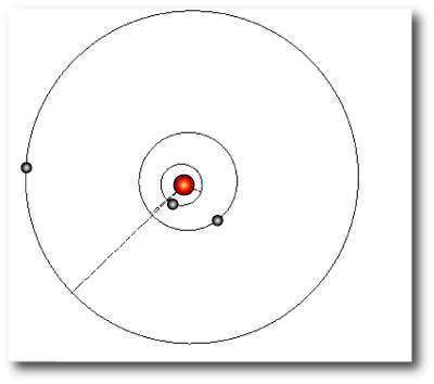
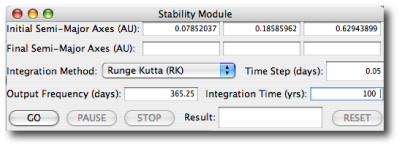
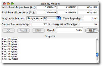
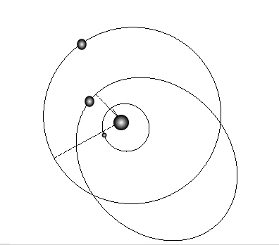
Among the eight entries that got both the total number of planets and their periods correct, there was a fair amount of variation among fits that had nearly equivalent values for the chi-square statistic. Chuck Smith (among others) turned in a configuration that bears a very strong resemblance to the actual input system. The four planets in his fit all have nearly circular orbits:
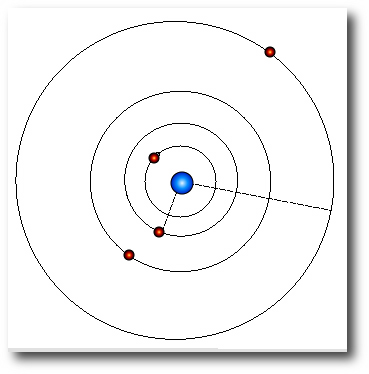
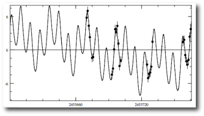
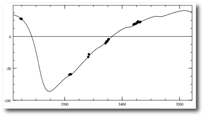
and the resulting radial velocity curve does a very good job of running through the data, with a chi-square value for the integrated fit equal to 1.1005:
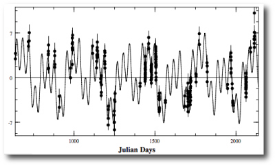
A number of other users turned in very similar configurations.
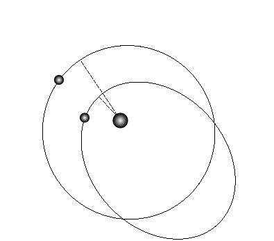
Because of random measurement errors in the data, the true underlying planetary configuration will not necessarily provide the best fit to a given set of radial velocity observations. Often, a better fit can be found for a configuration that is different from the system that generated the data. Steve Undy, for example, achieved a slightly lower chi-square value for his fit by giving a very significant eccentricity to his “Europa”:
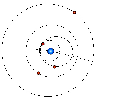
The winner of the contest, however, was Eric Diaz, who submitted a 6-planet fit that achieves an integrated chi-square value of 1.04. In addition to the four planets that are actually present in the model, Eric added small planets with periods of 1.06 days and 18.11 days. These objects soaked up some of the residual noise in the fit, allowing for a lower chi-square value, and a copy of the Sky and Telescope star atlas. Nice job Eric!
The contest raises some interesting issues. First, at what point should one stop adding planets to a fit? The chi-square statistic penalizes the inclusion of additional free parameters in a fit, but it’s clear that chi-square can nearly always be lowered by adding additional small bodies to the fit. Second, its very encouraging to see that subtle, but substantially non-interacting systems can be pulled out of radial velocity data sets. In this system, the masses of the planets are small enough so that their dynamical interactions with eachother are not significant over the time-frame that the system is observed. This is in stark contrast to systems such as GJ 876 and 55 Cancri where it is vital to take interactions into account (by fitting with the integrate button clicked on). Finally, I think that we’ll soon see examples of the 1:2:4 Laplace resonance as competitive fits within the existing catalog of radial velocity data sets on the systemic backend.


