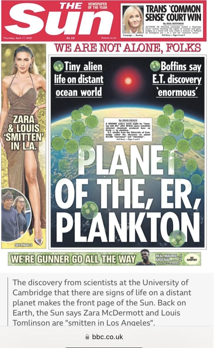
I used to tell my Ph.D. dissertation students that if you stick it out with the astronomy, the odds are fairly high that at some point you’ll get swept up more or less randomly into a Warholian vortex of notoriety. That phenomenon was certainly on display week before last when a formerly obscure researcher at Cambridge University pyramided his bumpy JWST spectrum into dimethyl sulfide and an algae-covered world that merited push notifications across the global media ecosystem.
My own fifteen minutes arrived back in January 1997 when Fred Adams and I were tapped to do an American Astronomical Society press conference on the End of the Universe. At the time, my mind was appropriately blown when I looked out at that modest sea of reporters and cameras. It was surreal to contemplate that a two-decade drought in press mentions that had begun with the 1977 story in the Champaign-Urbana News Gazette about how I’d been named Paper Route Carrier of the Month had abruptly ended with me holding forth about the Dark Era on the front page of the New York Times.
Charged with youthful energy, I was able to parlay that 1997 story into a multi-year stop-n-go career on the swampy fringes of public intellectualism. A museum talk with Philip Glass about the “music of the spheres”. A History Channel episode on the speed of light that featured a segment with some Shot Show promoters at a gun range in the Inland Empire. Extended back-and-forth wrangling over whether or not ‘Oumuamua is made of hydrogen ice.
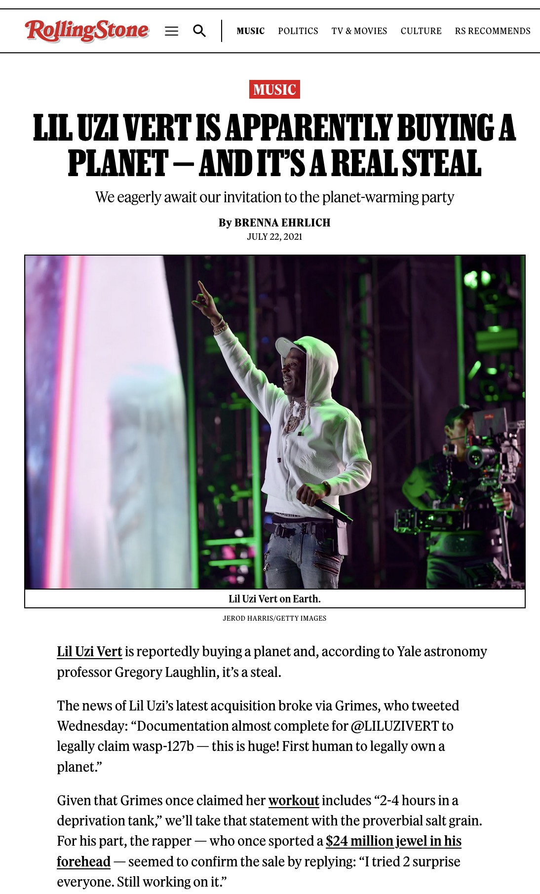
What I’m proudest of, though, is that I ended my run on the pages of Rolling Stone in the company of Lil Uzi Vert.
On Friday, a glossy eighteen-wheeler stretched its deluxe 75-foot frame along the prime High Street parking spaces across from Harkness Tower and adjacent to Yale’s Old Campus courtyard. “Black Elm Productions” was embossed on the side of the double-stacking Kenworth Cab.
Hey, that’s gotta be associated with the Spring Fling, I realized. I got out my phone and went to the Yale Daily News to find out who would be headlining this year.
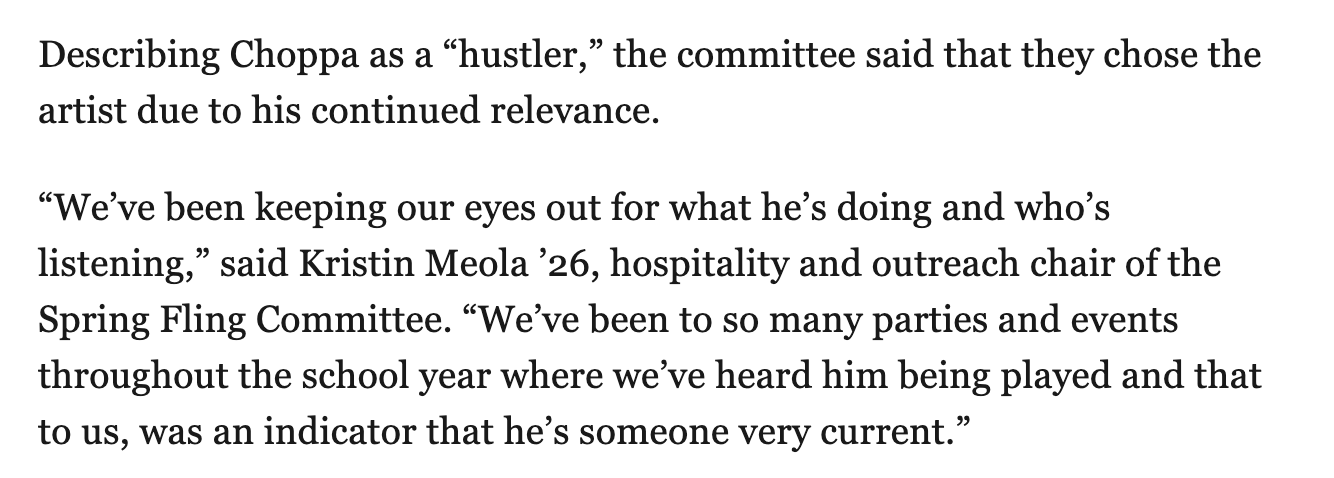
Bring ’em out. Bring ’em out… like everybody else, I like hearing some rim-rattling Glocks ‘n Gucci flow from the Dirty South. But I’ve never really managed to progress beyond my late-aughts cultural touchpoints. T.I. — What You Know. Rick Ross — Port of Miami. Young Jeezy. Now that it’s literally the year 2025, I’m literally like some mesozoic insect caught in amber. I’d never even heard of NLE Choppa, not to speak of never having heard Shotta Flow.
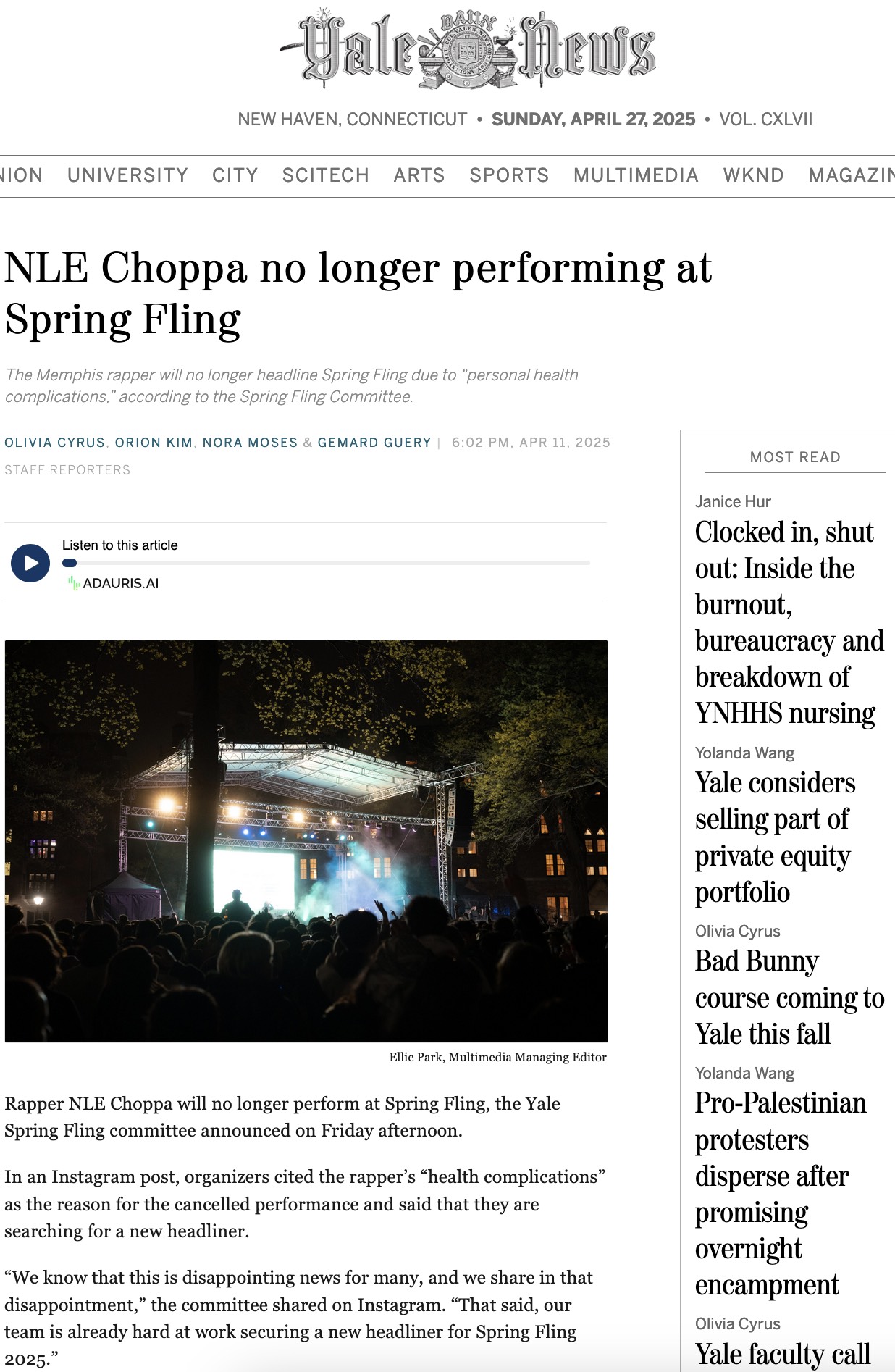
When I got home, I was wiring up the subwoofer so that I could get a bead on Choppa’s merits when I was informed that I’d missed a recent update from the Yale Daily News.
Some additional web-searching revealed how the committee had wound up handling the blow.
Ken Carson? WTF? Sounds like somebody that would have been opening up for Toby Keith.
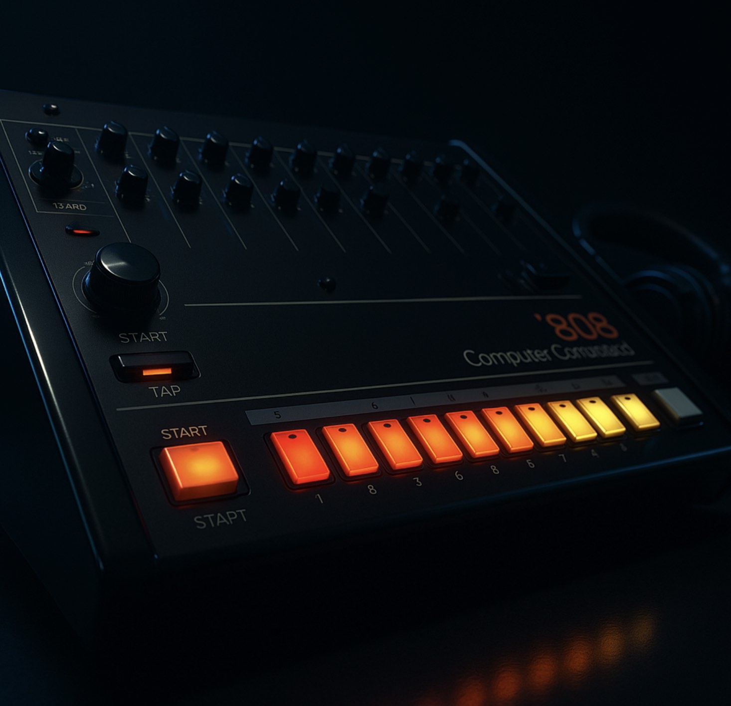
My initial concerns, however were, thankfully, entirelyunfounded. Check out the way the ‘808 drops in right at 2:10 of Blakk Rokkstar. That’s just about the most amazing thing I’ve ever heard.
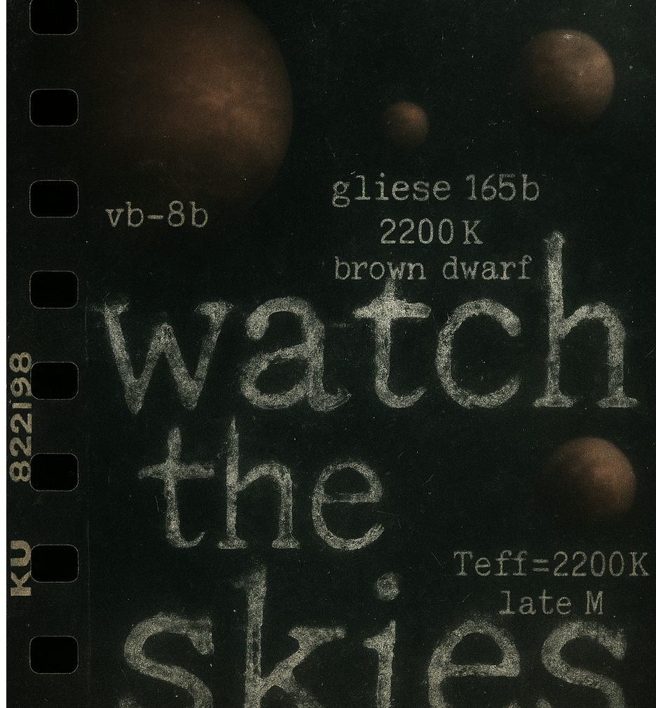
In 1991, brown dwarfs had a sketchy reputation. They were variously held responsible for everything from killing the dinosaurs to preventing the galactic rotation curve from decreasing in a sensible manner. A few years prior, there had been a high-profile discovery of the “first” brown dwarf, VB-8b, which was spotted orbiting VB-8 — a low mass red dwarf twenty-one light years distant that is part of the nearest known quintuple star system.
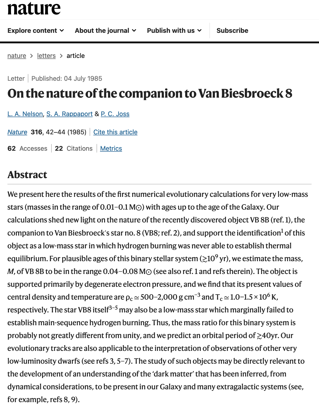
That generated a lot of excitement, a lot of analysis, even a conference. Here’s a Nature article that held forth on the cool new object. According to the abstract, the authors even racked up their own “first” (on the theoretical side):
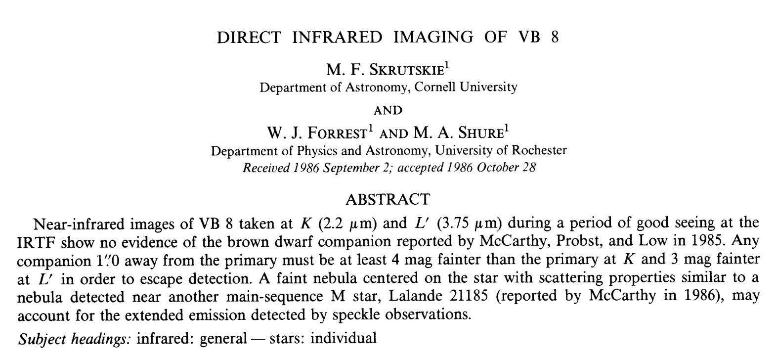
Unfortunately, however, VB-8b vanished upon further scrutiny.
The lack of any known brown dwarfs served to elevate their edgy mystery. The idea that one might actually be lurking in the near-solar neighborhood, nearer, perhaps than the closest stars, held a weird attraction. It was something I could glom onto. It was not like L1551.
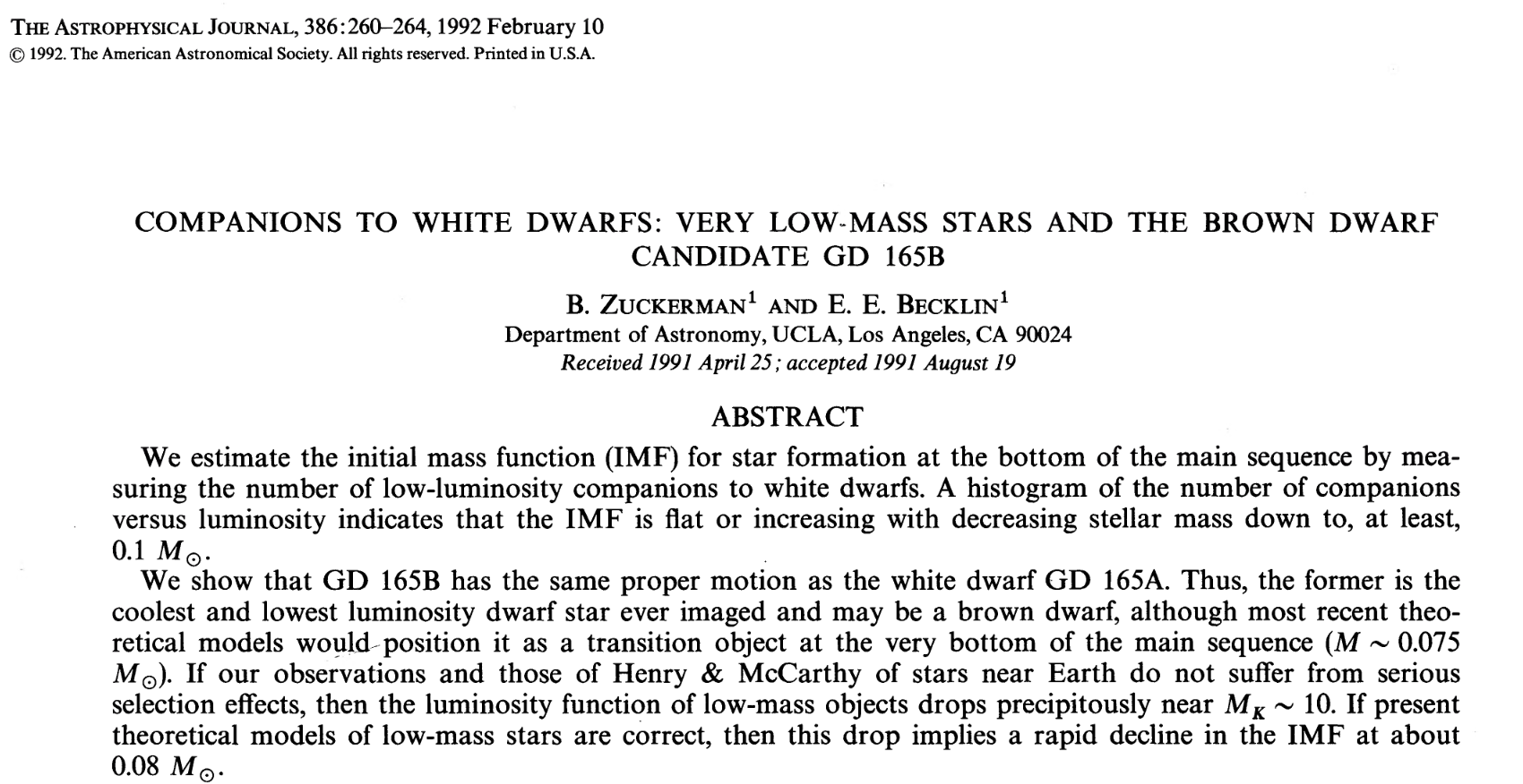
In August of 1991, there was a conference at UCSC on star formation, and one of the speakers was Ben Zuckerman from UCLA. I remember that it was a day when the thick coastal fog didn’t lift. Everything outside was gray and dripping wet. Zuckerman showed the results of different ongoing searches for brown dwarfs. I found myself suddenly snapped to attention. He was discussing the conclusions from a paper that they’d just gotten accepted and which was in press. It was eventually published in February of ’92.
The take-away was that brown dwarfs were probably very rare. That was a disappointment, and remarkably, given the lethargy I’d been showing toward astronomy generally, I was actually disappointed. I was surprised at how much I wanted the brown dwarfs to be looming out there. Preferably nearby.
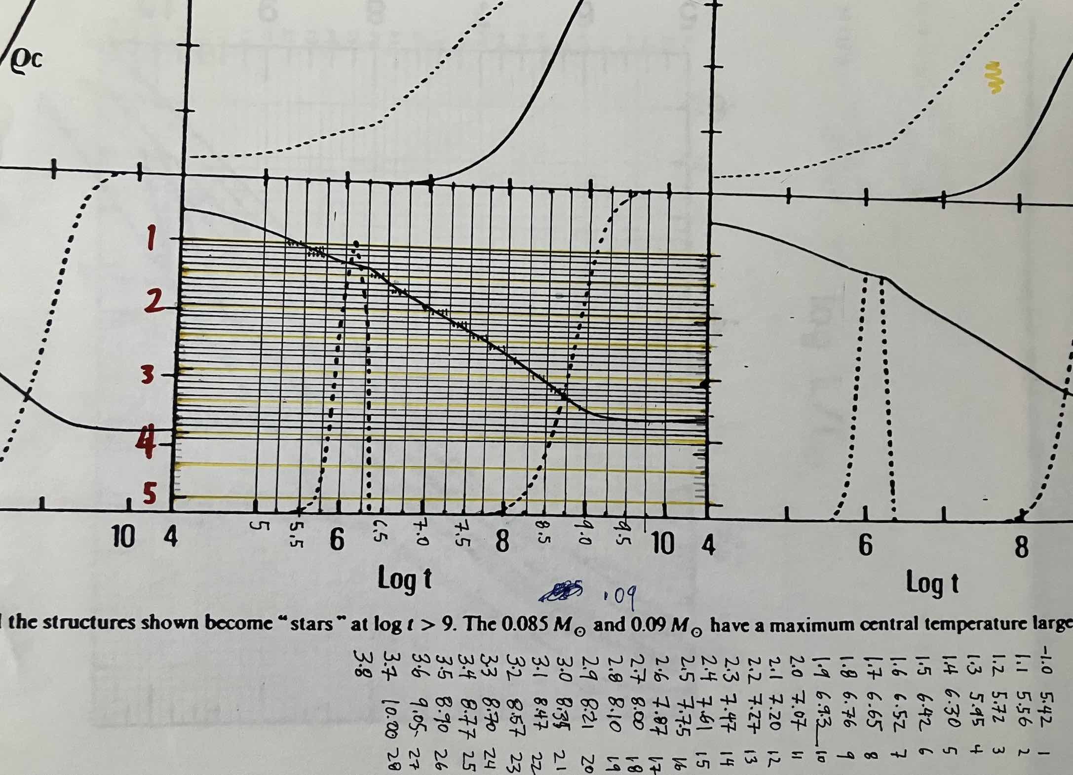
As Zuckerman showed his transparencies, I suddenly had a flash of an idea — maybe the first concretely independent and actionable idea that I’d had up to that moment. I had the intuitive feeling that the brown dwarfs weren’t showing up in the surveys because they were too dim. The cooling curves needed to be taken properly into account. They were out there, yes! but they were beneath the threshold of detection. And this was something moreover, that wasn’t just limited to a vague feeling. It could be calculated! I was galvanized into action. As soon as the session let out, I went to the Lick Observatory library to find the ingredients that I needed. Evolutionary models for low mass objects near the bottom of the Main Sequence. Bolometric corrections. The results of red dwarf surveys. I started working feverishly.
———–
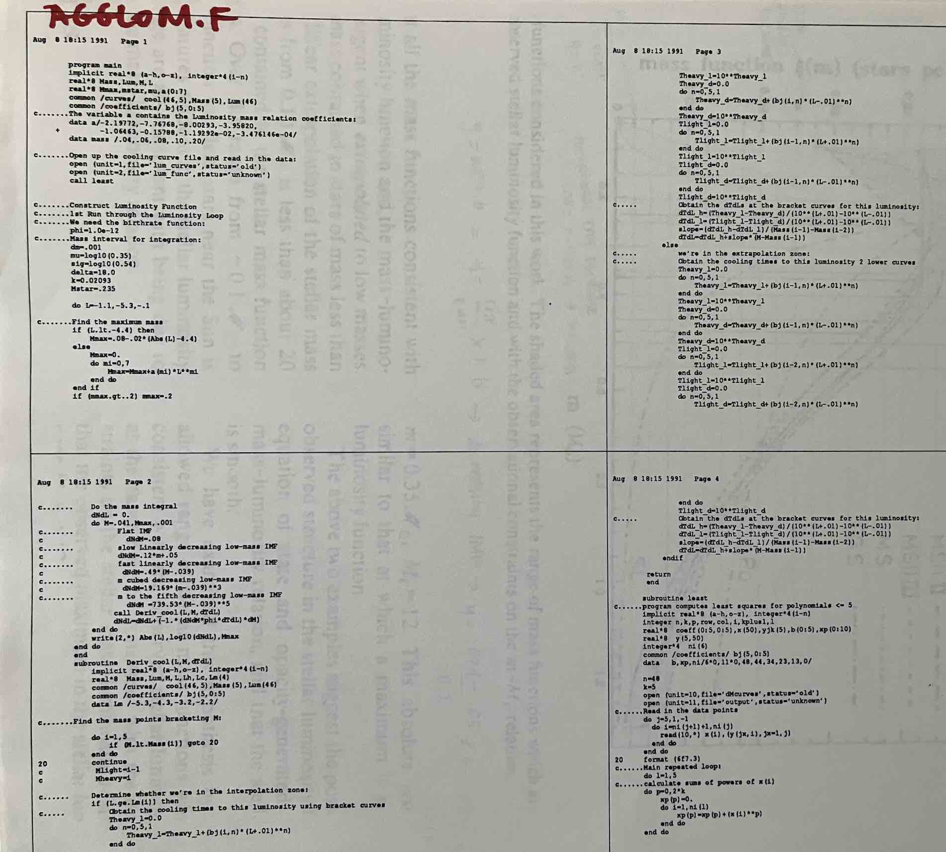
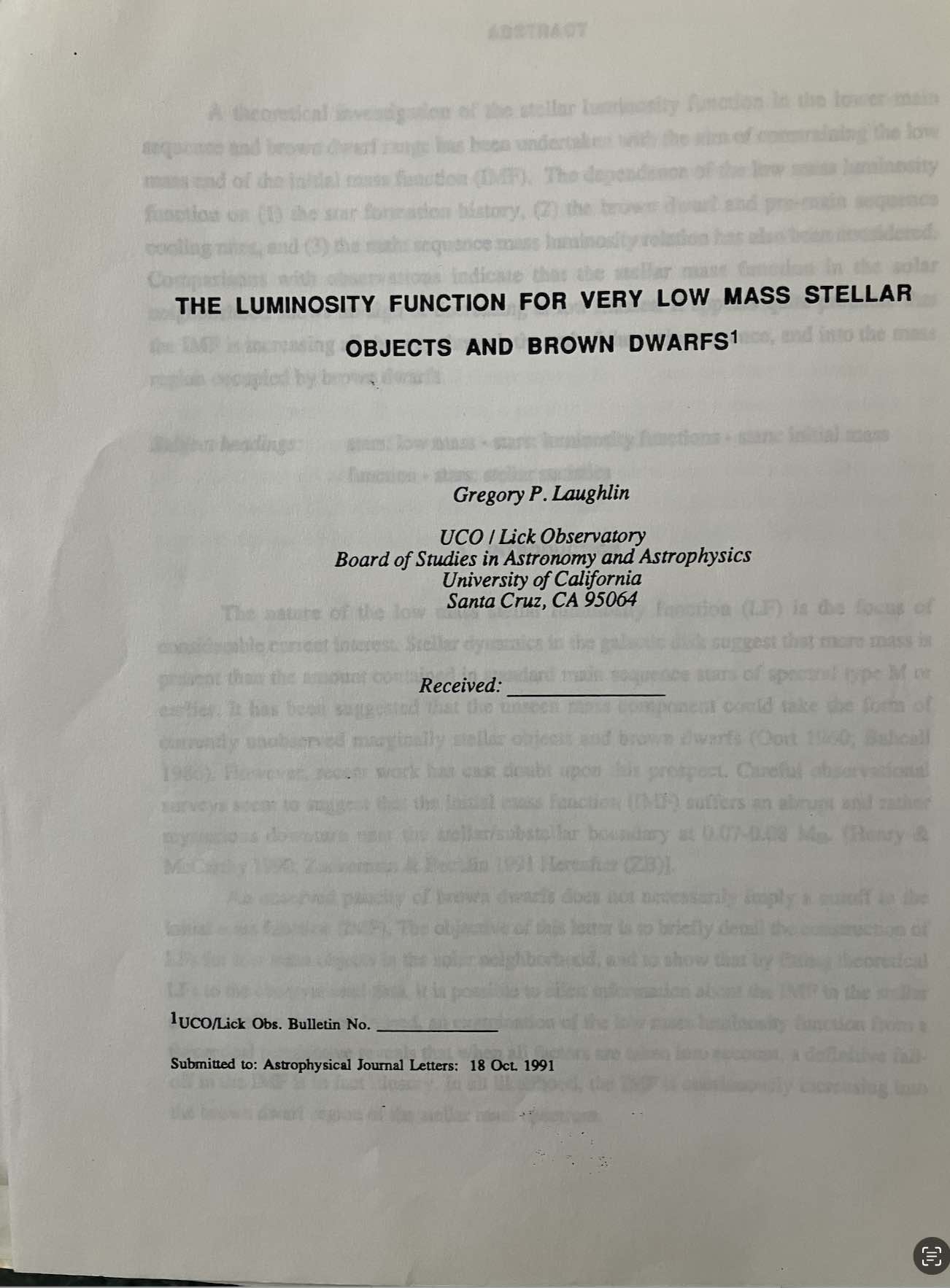
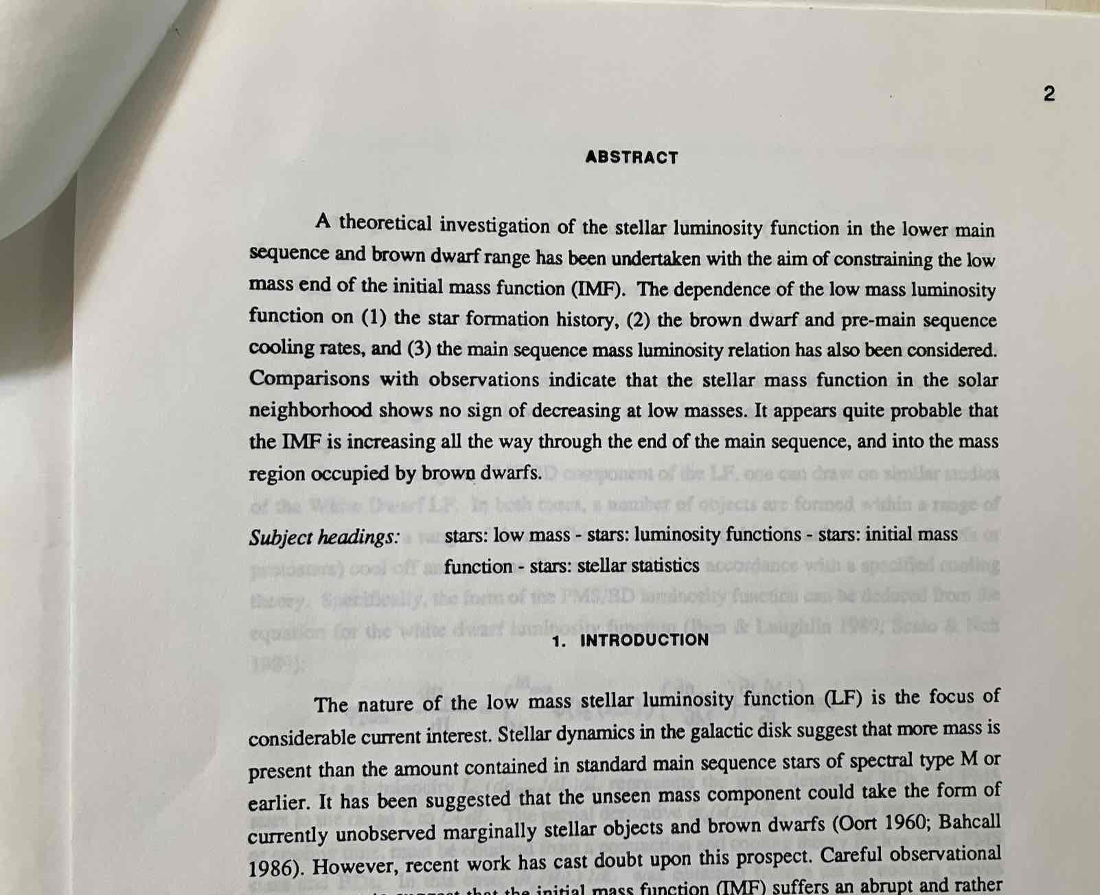
Recently, in going through old boxes, I found the notes from that effort, a time capsule from decades ago.
After several weeks, I had an answer. Even if the number of brown dwarfs per unit mass were increasing as one considered lower and lower masses, they would not be expected to show up in the extant surveys! I scrambled to write up a single-author paper. Peter Bodenheimer agreed that it was good enough to submit to the Astrophysical Journal Letters. It seemed to be the real deal.
I remember putting the final version in a mailing envelope and walking it to the post office. That was quite a feeling.
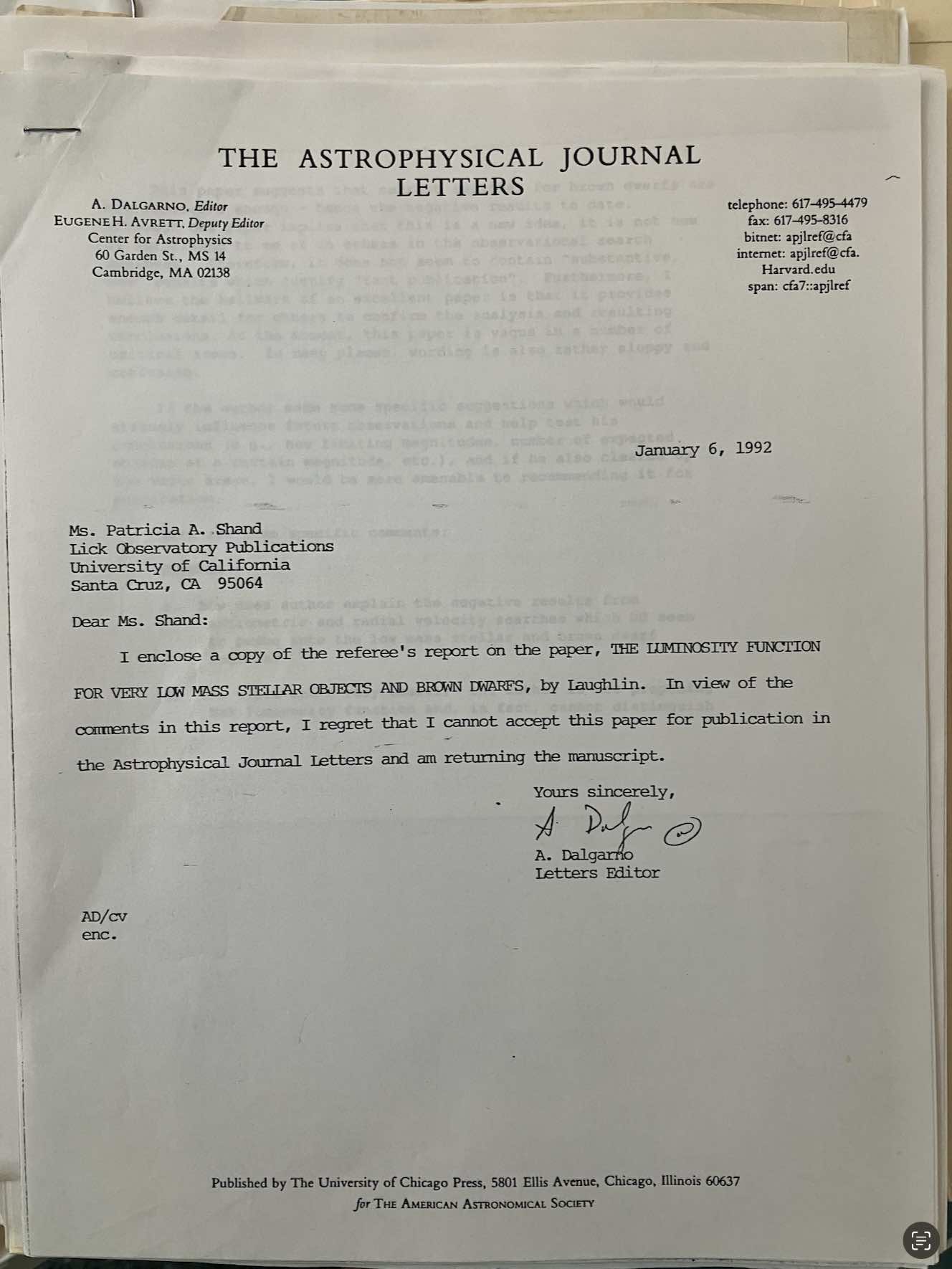
Almost three months went by. In January, one morning, the Observatory Director had placed a letter from Astrophysical Journal Letters in my mailbox. Heart pounding, I quickly opened the envelope.
The yellowing letter and the accompanying referee’s report still carry the dull remnant shock of rejection… “how does author explain the negative results from astrometric and radial velocity searches which DO seem to probe into the low mass stellar and brown dwarf regions?”, “wording is also rather sloppy and confusing”, “the title isn’t very useful” … and on and on.
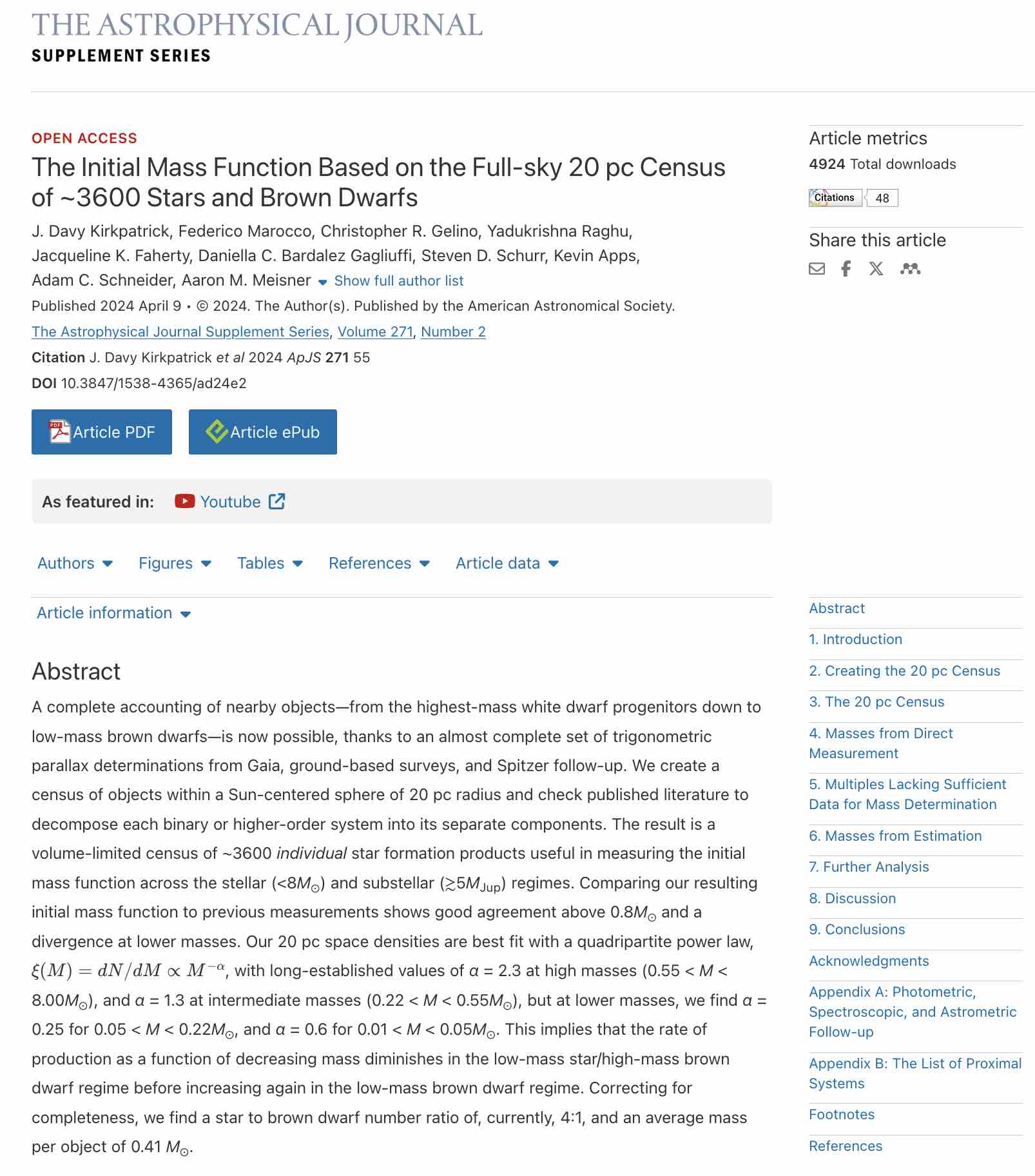
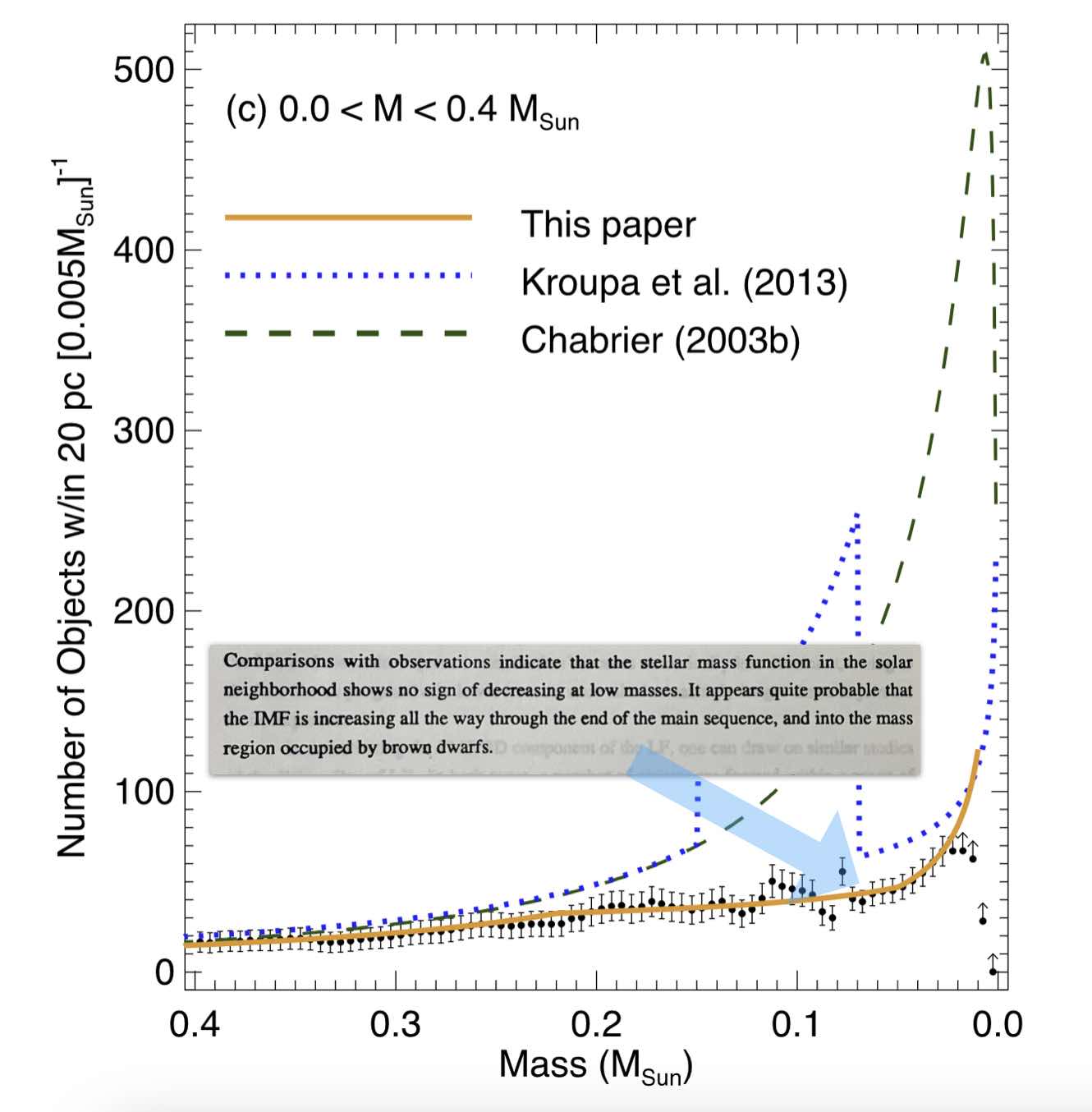
But the brown dwarfs are no longer so elusive. Thousands are known. I Iooked into the literature to see whatever happened to the mass function at the low-mass end. The most definitive treatment seems to be this article by Kirkpatrick et al. from last year:
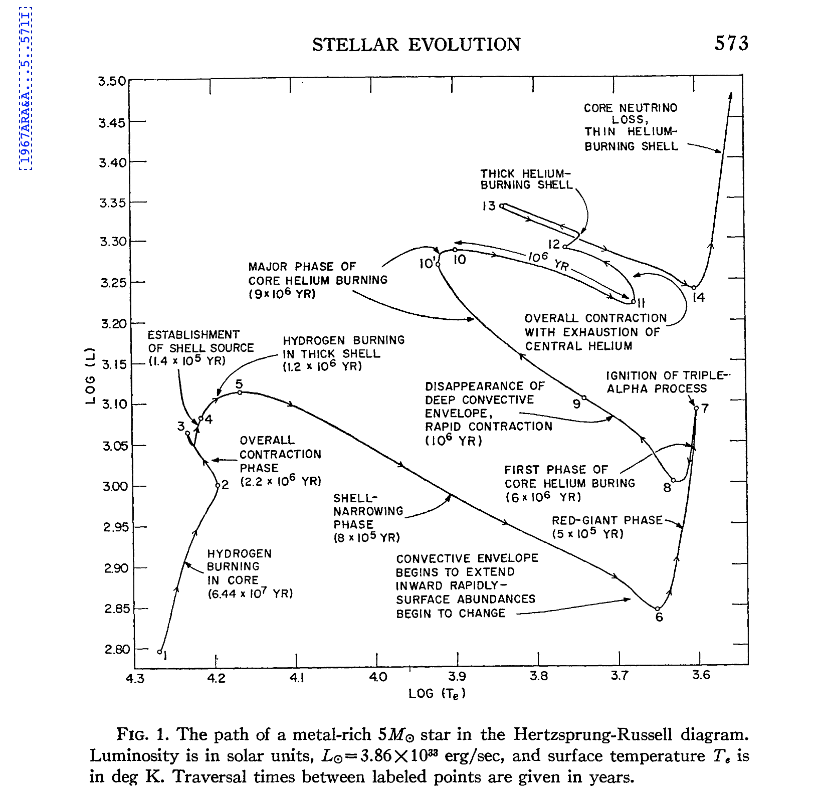
Brown dwarfs basically got the short end of the stick. At the start of the Nineties, the theory of stellar evolution was in very good shape. All of the genuinely relevant details regarding how stars work had been sorted out. If you did research on stellar evolution, you were engaged in the process of tying up loose ends. That state of affairs was possible because stars are essentially one-dimensional functions of radius. Spherical symmetry. Plots like this one from Icko Iben’s 1967 Annual Reviews article are emblems of a dramatic scientific success story.
With stars solved, brown dwarfs were on deck to be discovered and savored, and then it would be time, at some distant point, to start discovering extrasolar planets. Actual planets orbiting actual nearby stars — in 1991, that was a heavy concept.
That wasn’t how things turned out. The first bona-fide brown dwarf and the first HoJo were both confirmed in 1995. Look ’em up! The first exoplanet orbiting a bona-fide star, moreover, was discovered at 150-sigma statistical significance, which opened up the floodgates, led to a demand for ever-smaller planets at ever-smaller signal-to-noise, public outreach, explainer podcasts, and ultimately the dramatic conclusion to that age-old quest — the discovery last week that we are not alone.
August 1991. I was making no evident progress toward my career goals. I was fronting an industrial band in the derivative vein of Skinny Puppy and Front Line Assembly. We’d been essentially driven off stage during a recent show at the Kennel Club in San Francisco, in part because we weren’t very good and in part because we insisted on running both the SM-57 vocal mic and the bass guitar through an over-driven pre-amplifier before routing the signal to the house board. Our record had just come out, but it wasn’t moving units. Disconcertingly, I’d just heard No Depression from Uncle Tupelo, and the first bars of Factory Belt had triggered the inexorable erosion of enthusiasm for the industrial stylings of Bill Leeb and Nivek Ogre.
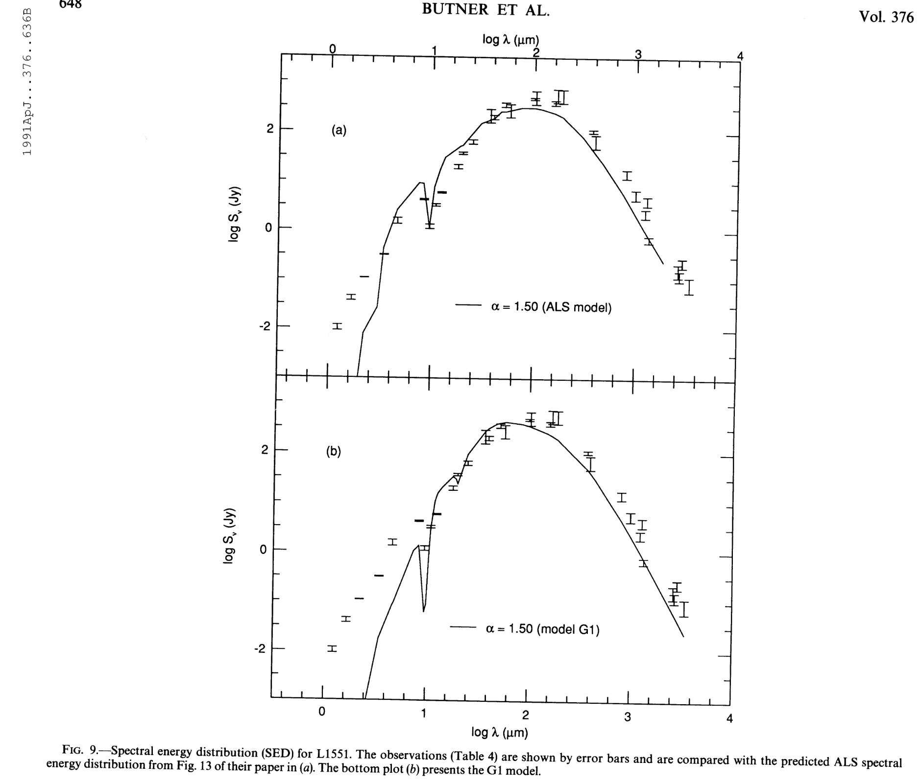
My astronomy research was also stalled out. I was supposed to be taking output from a hydrodynamical simulation of molecular cloud collapse and using it as input to a radiative transfer code, which would then create a fit to a spectrum of something called L1551.
The radiative transfer code generated points that were to be connected into a solid line which could then be plotted to compare with the observations of L1551. The idea was to get a line that was at least as good as the lines that had been published.
In retrospect, my total lack of progress is easy to diagnose. I had zero mental image or investment in what was going on. I didn’t care about L1551. I knew in the abstract what an infrared spectrum was, but I had no order-of-magnitude feel for it.
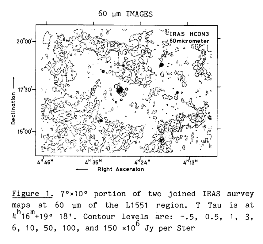
The crinkly 60 micron contour maps of L1551 bring to mind a segment from a 1981 interview of William S. Burroughs, in which the interviewer, Slyvere Lotringer, showed him a copy of a speech by Ulrike Meinhof on “Armed Anti-Imperialist Struggle”
“… Reality can only be perceived in a materialist way related to struggle — class struggle — war… The Guerilla has no real viewpoint, no basis from which to operate. Everything is constantly in motion, so is the struggle. Struggle comes out of motion, moving on and is moving on. All that matters is the aim. The Guerilla perceives class struggle as the basic principle of history and class struggle of history and class struggle as reality, in which the proletarian politics will be realized…
Burroughs quickly leafed through Meinhof’s tract and put it down impatiently.
WILLIAM BURROUGHS: I can’t visualize anything when I read this kind of material. I don’t see what it corresponds to.
I’m partial to that genre of articles where they detail the over-the-top morning routines of over-the-top productive go-getters. Like Mark (formerly Marky Mark) Wahlberg, who gets up at 2:30 AM for a big weight session followed variously by cryotherapy, prayer, supplements and intermittent fasting. That’s pretty bad-ass, you’ve gotta admit.
I set myself the challenge to write an Oklo post each day for thirty days in a row. It’s just over a week in now, and it’s starting to show. I’m gonna hit the sack now and schedule this post to show up at 2:30 AM.
No denying it, Edward Tufte’s The Visual Display of Quantitative Information was a seminal book, and the follow-ups, in particular, Envisioning Information, were remarkable as well. I was exactly the right age to absorb them when they came out. Some of Tufte’s lines are just classic:
… A series of weird three-dimensional displays appearing in the magazine American Education in the 1970s delighted connoisseurs of the graphically preposterous. Here five colors report, almost by happenstance, only five pieces of data (since the division within each year adds to 100 percent). This may well be the worst graphic ever to find its way into print ...
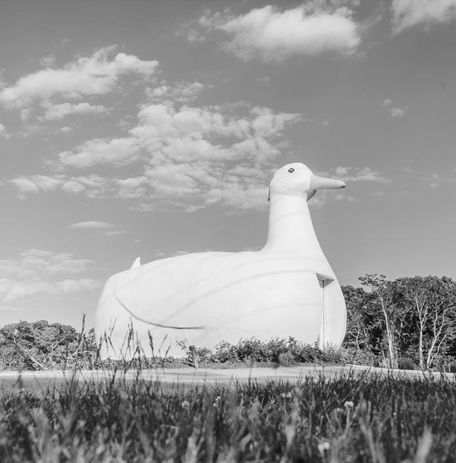
That paragraph falls in the midst of admonitions against self-promoting graphics. Tufte callssuch constructions Ducks, where the reference is to the Big Duck Store on Long Island:
Tufte’s take-away, as explained in a quote (which itself is from a quote)that he pulls from Learning from Las Vegas, seems to be that is is all right to decorate construction but never all right to construct decoration.
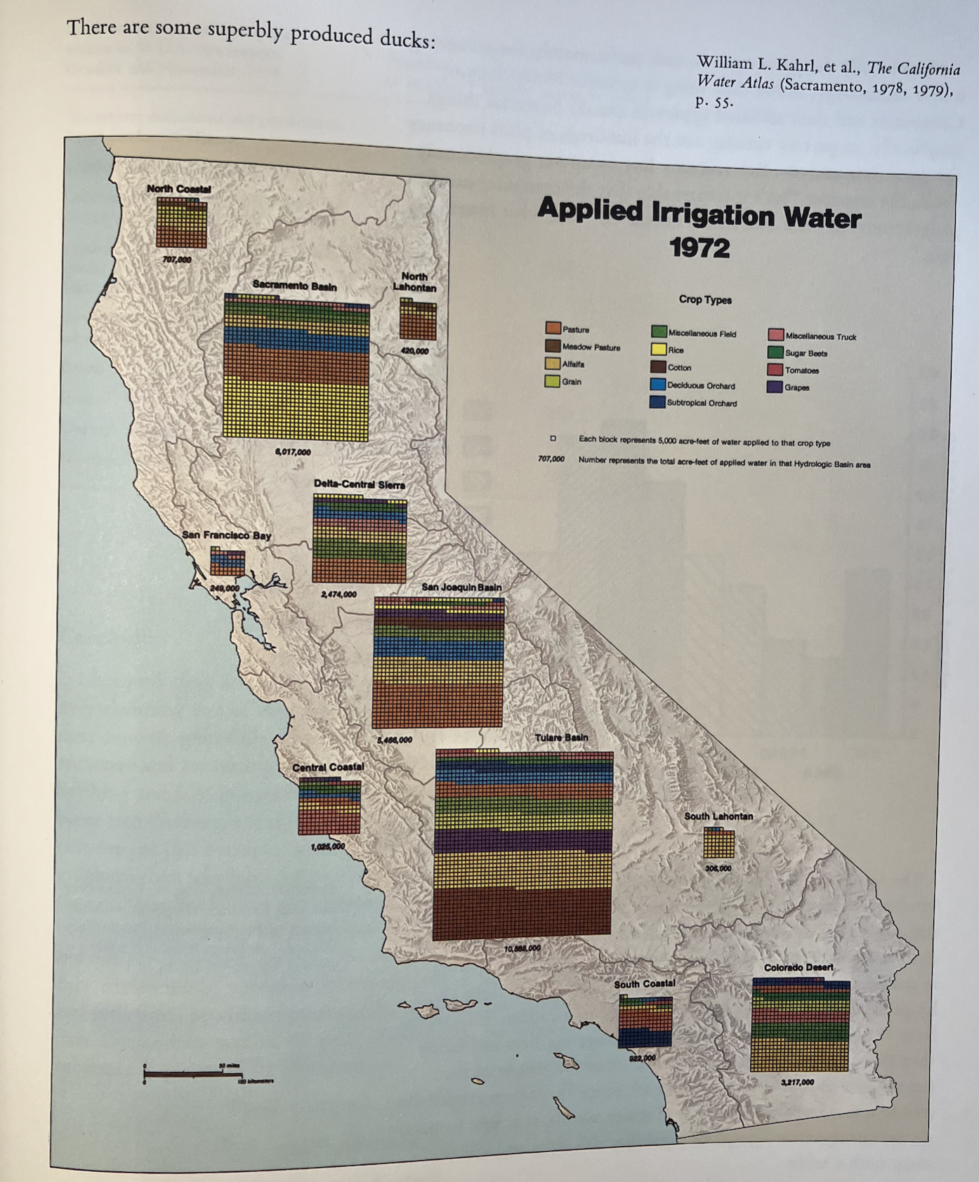
Sure, I’m fine with that. But then I’ve always been confused by p. 119, whose single line of text runs, ambiguously, “There are some superbly produced ducks:”
So clearly, p. 119 seems intended to serve as another admonition, yet that graphic doesn’t strike me as bad at all… In fact it’s a great graphic that incorporates many of the stylistic choices (small multiples, etc.) that Tufte generally recommends. The net effect was to leave me feeling confused regarding exactly where I should properly hold forth and grandstand within the whole endeavor of data graphics.
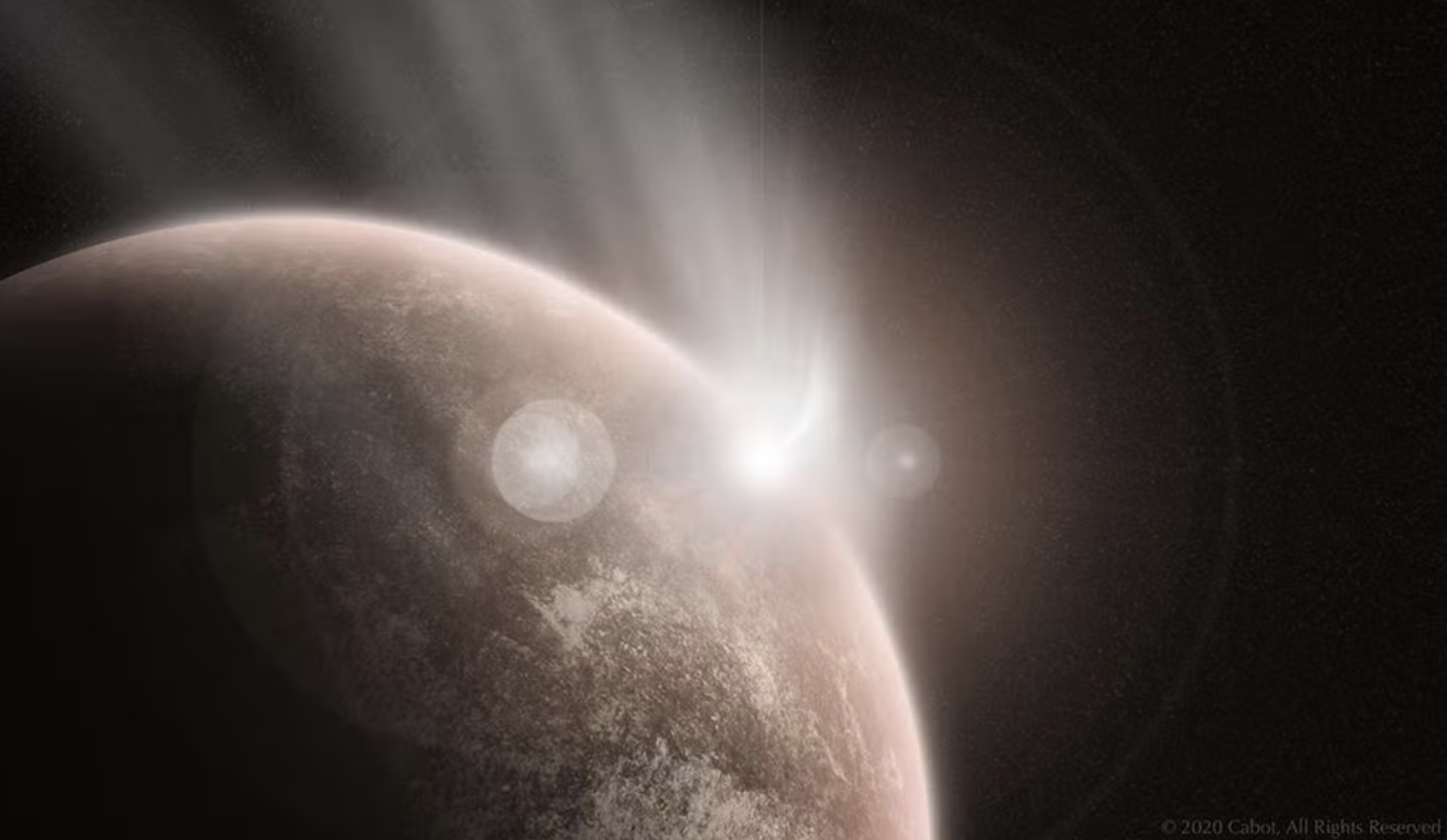
The splash image for this post is definitely a construct of decoration. It was constructed by Sam Cabot using his black-belt photoshop skills for the purposes of decorating our self-promotional press release. It strives for photorealism of a KT-style impact on Venus, back when Venus had a one-bar atmosphere, oceans, life, maybe a civilization, etc. What does the moment of impact actually look like?
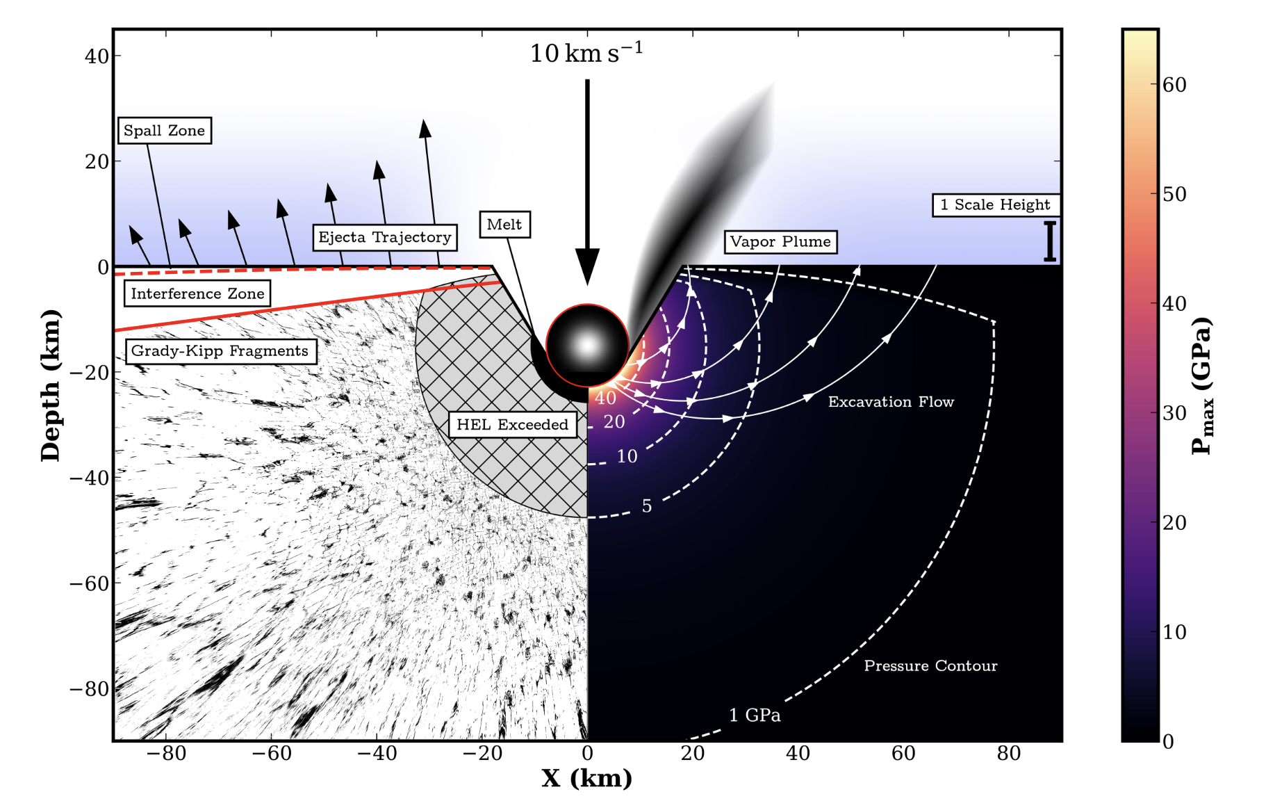
In the paper itself, we have another graphic that Tufte would probably dismiss as a duck:
It serves to fix ideas regarding the impacts that could have transferred huge amounts of material from Venus to the Moon, where they’re now churned up in the lunar regolith, waiting to be analyzed and discovered, and chewed over in a few upcoming posts.
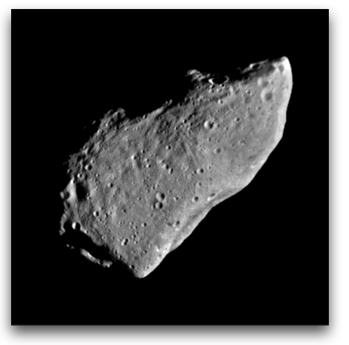
On October, 29th, 1991, the Galileo probe, flying through the Main Belt on its way to Jupiter, approached within 990 miles of 951 Gaspra and radioed back the first up-close view of an asteroid — a tiny world too small to be round. I was in graduate school at UCSC at the time. At the beginning of November, a glossy black and white clay-coated photograph showing the view above was tacked to the Departmental Bulletin Board. It had been sent direct from JPL in appreciation of Arnold Klemola’s work on the stellar ephemerides that had permitted the flawless navigation of the close approach. The Mosaic Browser hadn’t yet appeared. I remember staring at the physical photograph for a long time.
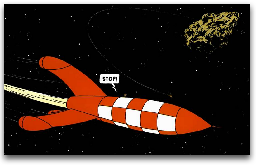
When a new type of celestial object is first seen in detail, surprises usually result. Gaspra, however, seemed to conform to the popular impression of what an asteroid should look like. I remember thinking how the depiction of the near-Earth asteroid Adonis in Herge’s Explorers on the Moon (1952) had wound up being rather on-the-mark.
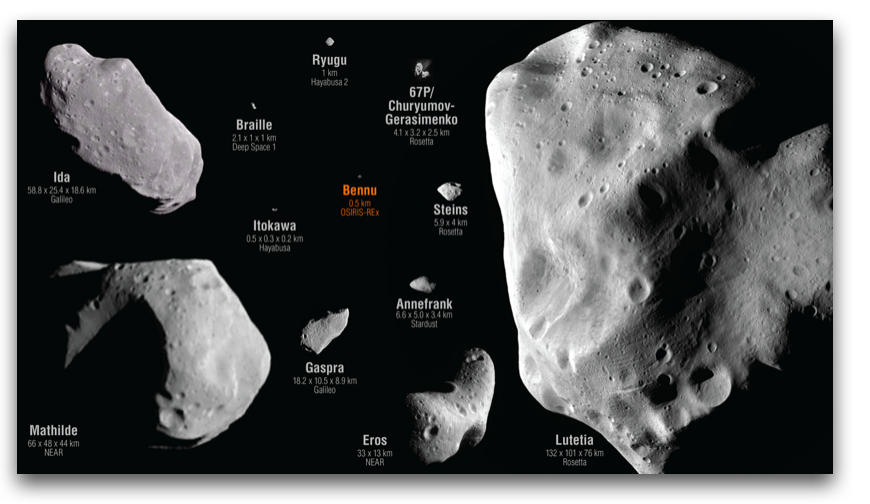
Over the past three-plus decades, spacecraft have visited a whole raft of additional asteroids. The album of returned photographs is a classic of scale invariance in that the images of the asteroids offer almost no clue to their true sizes. It’s a little jarring to see them arranged with their accurate relative sizes, where 14,000 Bennus make a Gaspra and 600 Gaspras comprise a Lutetia.
Uncertainties regarding the true sizes of asteroids would thus seem like a less than front-burner concern. The exact size of this or that particular body would be of enormous interest if it were determined to be on a collision trajectory, but otherwise would presumably be of minor consequence. What you’d think would be a sleepy topic, however, somehow managed to roil into controversy that generated New York Times articles and FOIA requests.
The cherry blossoms this weekend had me recalling moments from the year I spent in Japan.
While I was there, I visited Hokkaido University in Sapporo to give an colloquium. After a day or so, it began to dawn on me that an odd motto, “Boys, Be Ambitious!” is attached (in English) with great frequency to the various affairs both large and small of the University. One of the astronomy graduate students had the phrase written on a post-it note attached to the screen of his computer. In another building, there was a large mural showing a stern, stiffly dressed 19th-century gentleman exhorting a group of reverent students with a longer version of the phrase:
“Boys, be ambitious! Be ambitious not for money or for selfish aggrandizement, not for that evanescent thing which men call fame. Be ambitious for that attainment of all that a man ought to be.”
Which upon reflection, seems to be excellent advice…
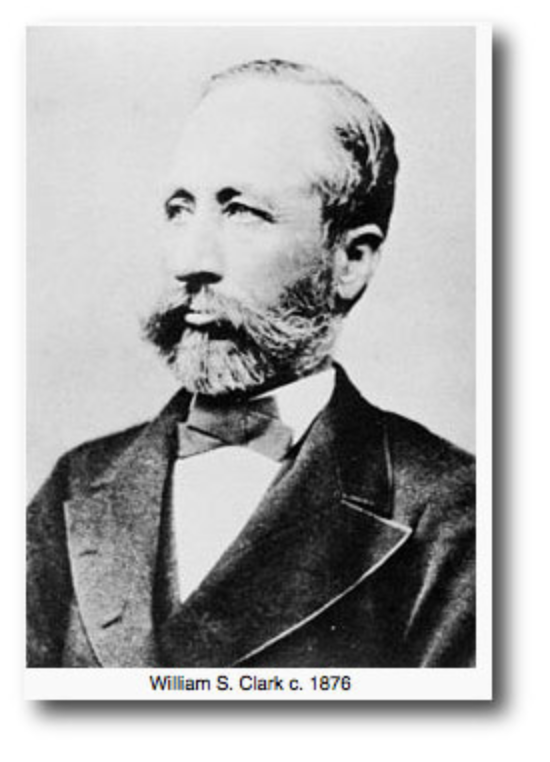
The gentleman in the mural, it turns out, is William Clark Smith, the founder and first president of the University of Amherst, Massachusetts. In the mid 1870s, he was enlisted by the Japanese Meiji Restoration government as an Oyatoi Gaikokujin, or “hired foreigner”, to establish an agricultural college in Sapporo (now Hokkaido University) and he made an impression that lasted well over a century. His Wikipedia article is extensive and quite interesting. On the origination of the motto:
“On the day of Clark’s departure, April 16, 1877, students and faculty of SAC rode with him as far as the village of Shimamatsu, then 13 miles (21 km) outside of Sapporo. As recalled by one of the students, Masatake Oshima, after saying his farewells, Clark shouted, “Boys, be ambitious!”
Upon returning to the United States, and flush with the organizational successes and appreciation that he had garnered in Japan, Clark left his academic career, cultivated an interest in gold and silver mining, and embarked on an abrupt, ambitious, and ultimately disastrous foray into the business world. In 1880, he teamed up with a junior partner, John R. Bothwell, to found what might best be described as a 19th-century incarnation of a metals hedge fund. From offices on the corner of Nassau and Wall Streets in Manhattan, the firm of Clark & Bothwell acquired interests in a slew of silver and gold mines across North America, for which they assumed management and issued stock. Clark, as president, got his contacts and colleagues to invest in the venture, and for a period during 1881, the stocks issued by Clark and Bothwell ran up into multi-million dollar valuations.
Clark traveled around the country, promoting the company, acquiring new mines, and seeing to their management, while Bothwell appears to have been responsible for back-office operations. Clark, who had no experience in finance, and little real knowledge of mining geology seems to have spun his wheels, while Bothwell, who had a shady history, actively mismanaged the companies. The operation got into debt, with the outcome being all too typically familiar along the lines of When Genius Failed. By the Spring of 1882, they were facing insolvency, investor lawsuits, fraud allegations, and various other problems. Bothwell disappeared on a train trip to San Francisco, never to be seen again, leaving Clark holding the bag. The story played out to the delight of the Massachusetts and national press.
From the Springfield Republican, May 29, 1882:
… it appears form the beginning that he, as manager of the mines has allowed Bothwell, as treasurer, absolute control of the books and finances of the several companies. It doesn’t appear that he ever examined the books, nor had anybody do so for him, or inquired into the financial condition of each mine, or what was being done with their profits; neither has he required from Bothwell such bonds as the latter’s position should require for the safe handling of moneys entrusted to him…
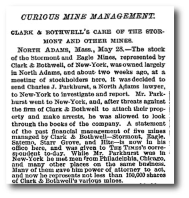
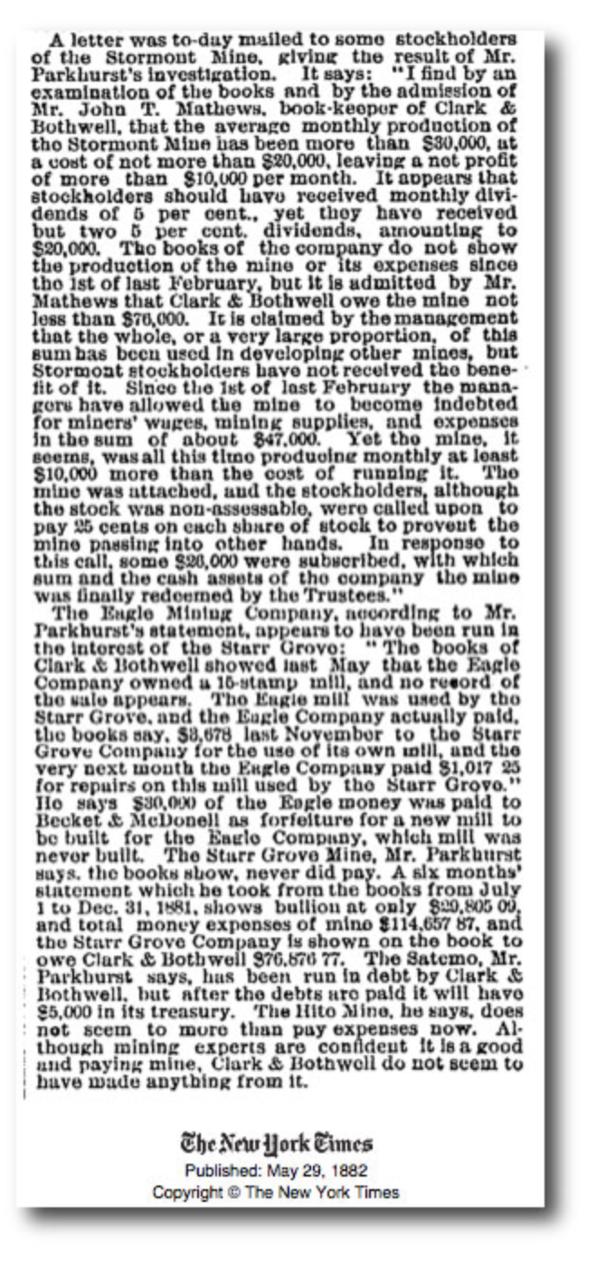
The scandal made the New York Times, which wrote several articles about the affair, including this one, from May 29th, 1882:
The scandals eventually ruined Clark’s health, and he died four years later, in 1886, at age 60.
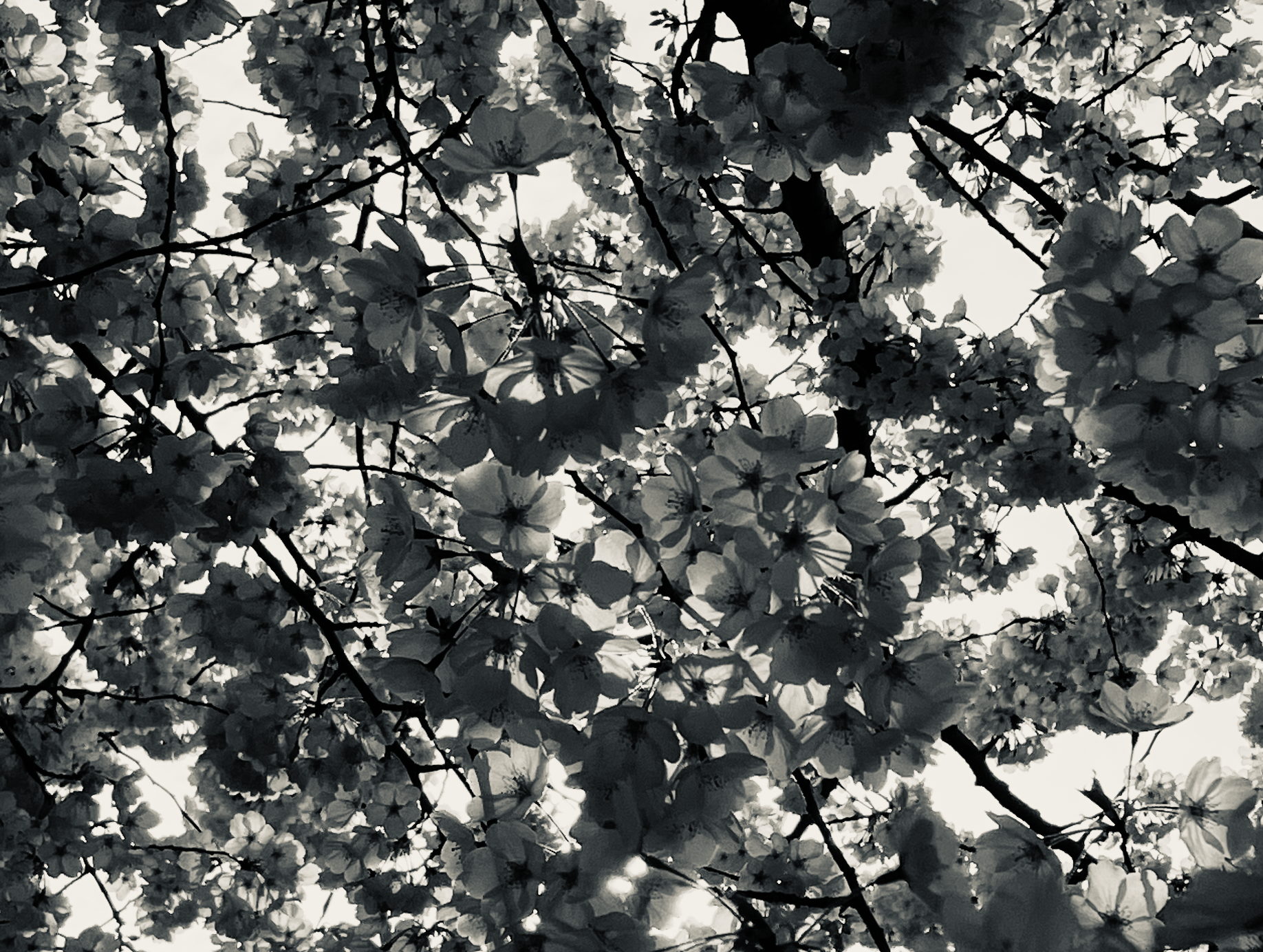
The cherry blossoms of Wooster Square looked like they’d reached their peak this morning. My anecdotal feeling was that they were at least one week late this year compared to the past several years.
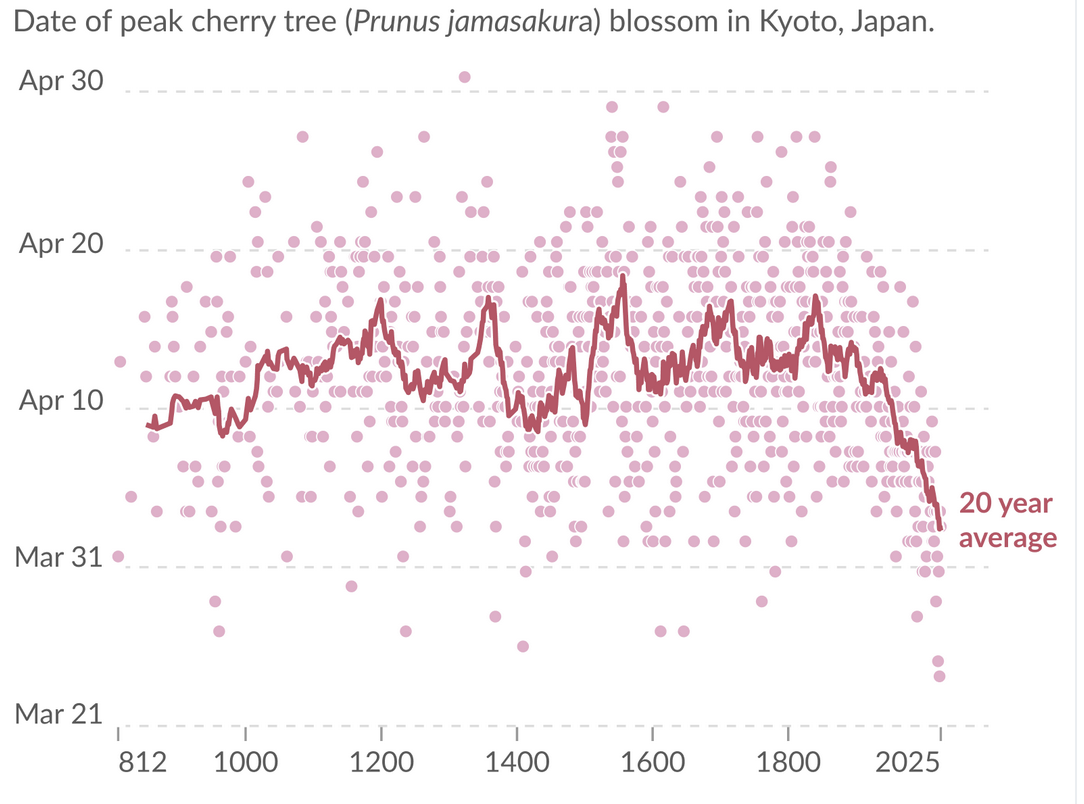
I know it’s cliche, but I’m drawn to the Kyoto cherry blossom peak date data set, which goes back to the year 812. This year, in Kyoto, the peak date was April 4th.
During the year that I lived in Tokyo, the cherry trees in Ueno Park reached their peak in early April. A week later, I went there on the crowded silent subway, but by that time, the sakura were mostly gone, a greying carpet strewn across the concrete sidewalks.
What’s the most interesting unanswered question in Solar System planetary science? Hands down, I’d argue it’s, Did Venus have oceans, and if it did, when did it lose them?
At first glance, Venus looks promising. It’s got essentially the same mass and radius as Earth. Now that the extrasolar planets provide context, Earth and Venus look like a “pod”, a consequence of the ill-understood process that permits a given system to repeatedly manufacture worlds that are near-clones. Sure, Venus is closer to the Sun. But the clouds reflect most of the light, and it was only in the 1950s that it became clear that perpetual overcast isn’t the only problem with the Venusian weather report.
The climate on Venus might not always have been so bad. The Sun was 30% less luminous at the start of its main sequence life, which means that the sunlight intercepted by Venus was once only 135% of the current terrestrial flux, the equivalent of moving from Detroit to Santa Monica.
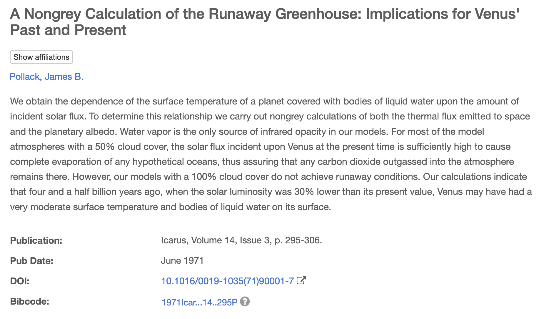
This 1971 paper seems to be the first spark of realization that we might have “lost” Venus at some point in the distant past.
From there, it’s not hard to let the imagination run away. Continents. Oceans. Primordial forests. A vanished alien civilization. All within the realm of far-fetched possibility. Dude! Snap back to reality. The hybridization of Occam’s Razor and Bayes’ Theorem states simply, “That super-cool hypothesis of yours? It’s wrong.”
Nonetheless, the question of whether Venus had oceans (and if it did, when it lost them) seems like it should be answerable. How does one make an approach?
It’s easy to think of long-shot ideas, and indeed, I’ve been semi-preoccupied with this question for the last twenty years. Take phosphine — there’s an idea I didn’t think of… If there’s phosphine in the Venusian atmosphere then that points to life, and if there’s life, it’s likely is a remnant holdout from pre-greenhouse oceanic days. A nice story! It’s wrong, of course (see the bold-faced statement above) but it’s beguiling enough that efforts are afoot to spend a lot of money to pursue it.
This blog is named after the Oklo reactors, which demonstrate that under certain special circumstances, the occurrence of uranium criticality can be discerned long after the fact… What if there was a ancient nuclear war on Venus? Are there isotopes or isotope ratios created by a critical assembly of plutonium or uranium that would produce a detectable signature after billions of years? As far as I can tell, the answer seems to be no. What about uranium hexaflouride? It doesn’t occur naturally, it’s the go-to molecule for effecting isotope separation, and it’d be a gas under Venusian conditions. Unfortunately, the acid aerosols in the Venusian atmosphere would clear it out in virtually no time if it were released. It wouldn’t be around a billion years later.
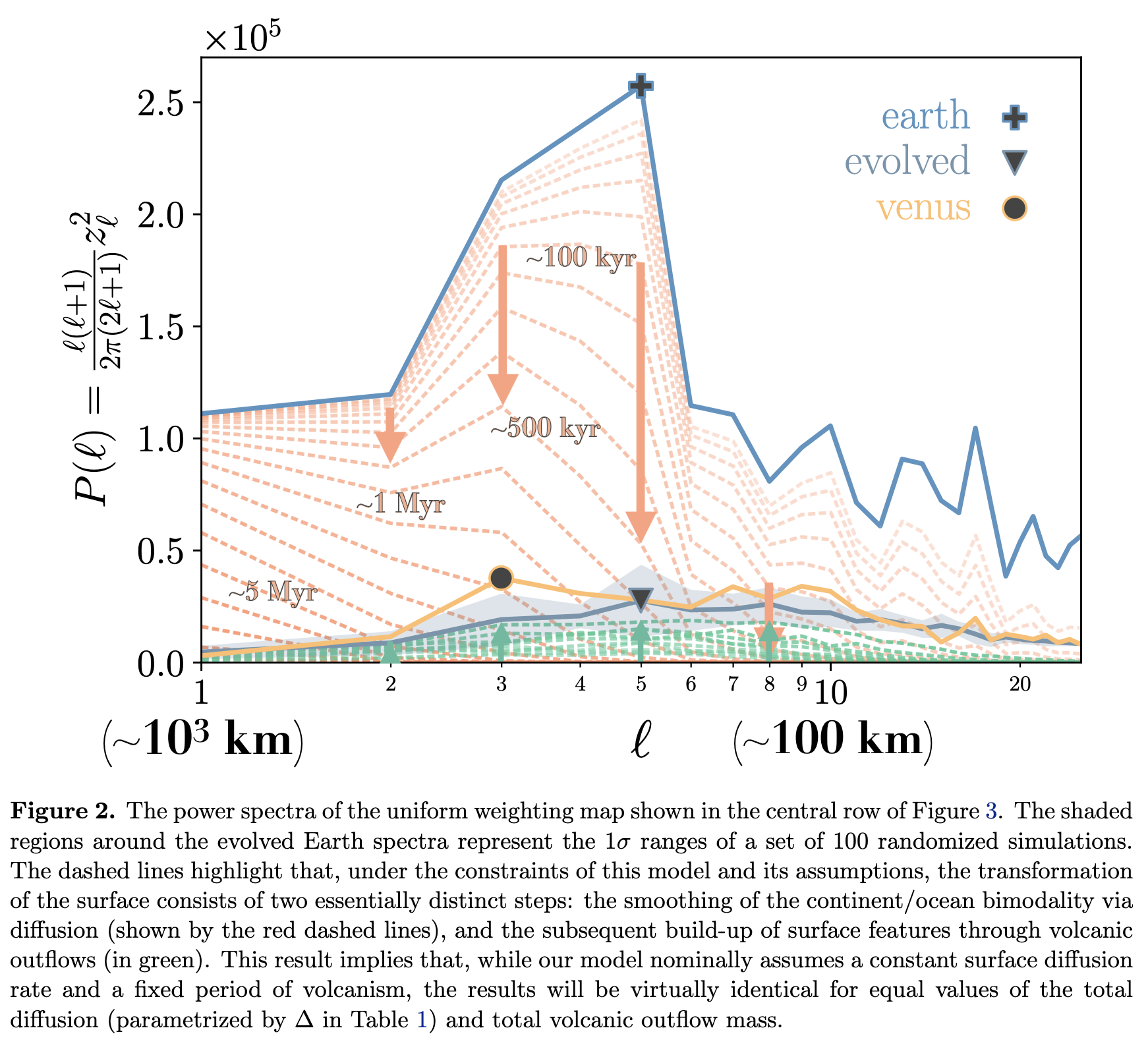
If you scroll down to read the posts from the past year, you’ll find there are several that touch on a more sober-minded approach to the lost oceans problem. The idea explored is encapsulated in this figure:
and the hypothesized sequence (which is pretty cool, so therefore very likely wrong, but not completely certain to be wrong) is as follows:
Venus had water oceans, an atmospheric pressure of order a bar, and plate tectonics.
Steadily increasing solar luminosity drove a runaway moist greenhouse.
Rapid erosion occurred as the oceans were being lost.
Erosion ceased and plate tectonics shifted to stagnant lid volcanism.
Lava from large igneous provinces created the current topography.
Using Earth’s lava production rate points to oceans being lost in the late pre-Cambrian.
Arthur Adams and I worked on this around the time of Covid. It was the subject of an arXiv preprint and a Caltech GPS Departmental Colloquium in March of ’23 :
The buzz was then killed by a daunting, demoralizing referee’s report that left the prospects for a peer-reviewed journal publication very much in limbo, and pointed to the need to find a new approach.
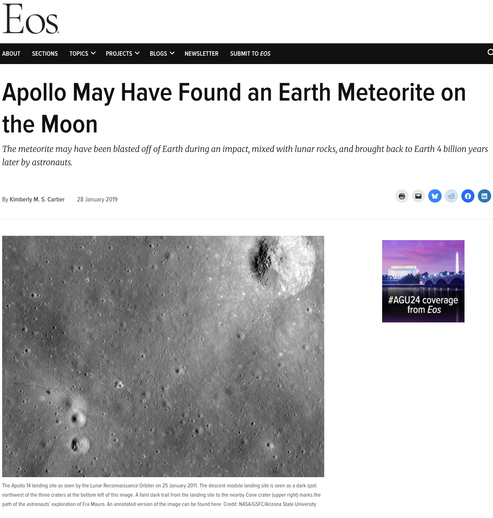
This article from caught my eye:
The Eos article is a popular-level summary of a 2019 paper by Bellucci et al. that reports the discovery of an unusual granite-like fragment, a “felsic clast” in one of the samples returned by the Apollo 14 Mission. The clast contains zircon grains with geochemical formation signatures—specifically formation in the presence of high oxygen availability, low crystallization temperature (~1500° F), and high-pressure (~6.9 kbar)—that are atypical for known lunar rocks but are consistent with Earth’s continental crust. These traits suggest the clast either formed under unusually oxidizing, volatile-rich conditions at a level of order 170km below the lunar surface, or alternately, originated on Earth at shallower depth and was transferred to the Moon by a large impact over four billion years ago. The article pushes for the terrestrial origin hypothesis, and because I’m not an expert, it looked pretty convincing.
Given that set-up, it’s natural to ask — what if the clast is from Venus?
It’s coming up on a decade since the Planet Nine announcement, and the Batygin-Brown article in the Astronomical Journal, has accumulated a remarkable 666,130 (and counting) downloads. To catch myself up, I’m working an overview for Oklo of where the situation stands.
To help encapsulate the process, I’ve made a playlist that strives to obliquely capture the narrative arc of exhilaration, hope, fear, resignation, acceptance, and ultimately optimism that it’s out there… the traces of its presence should already reside on the drives in the RAID arrays, suspended in the exabyte seas…
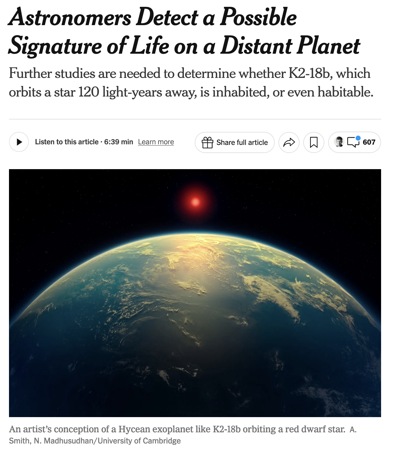
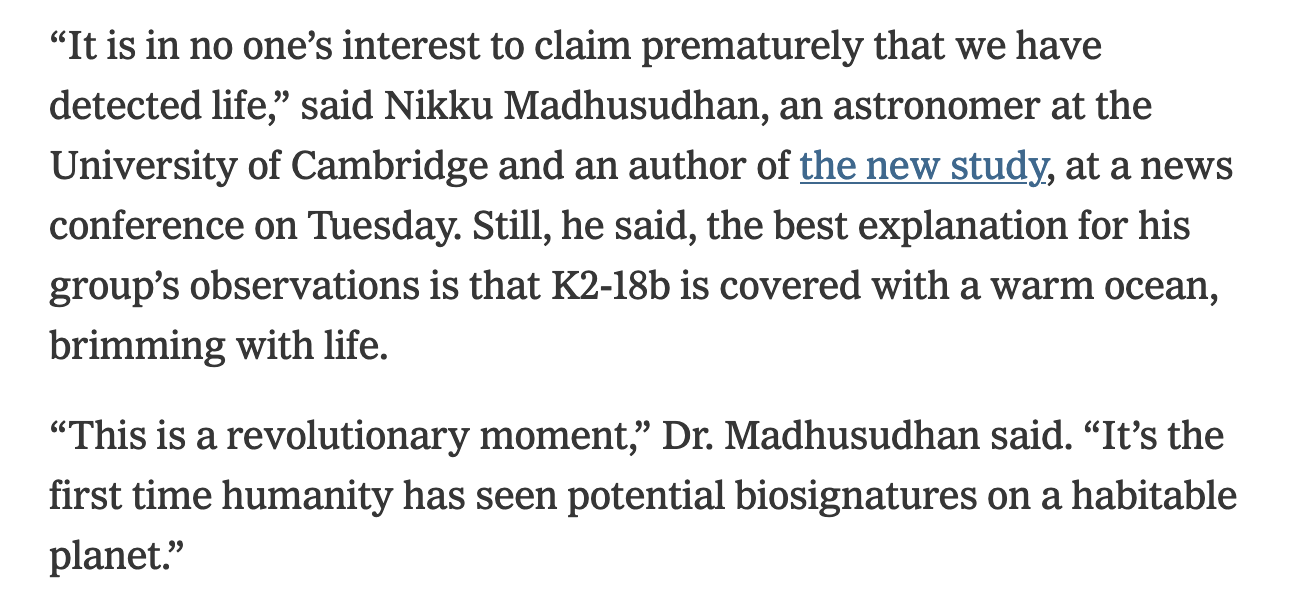
We were treated to the latest life-discovered-on-an-exoplanet story in this morning’s newspaper:
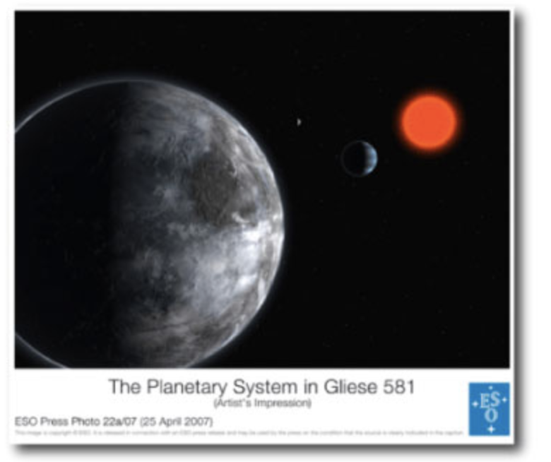
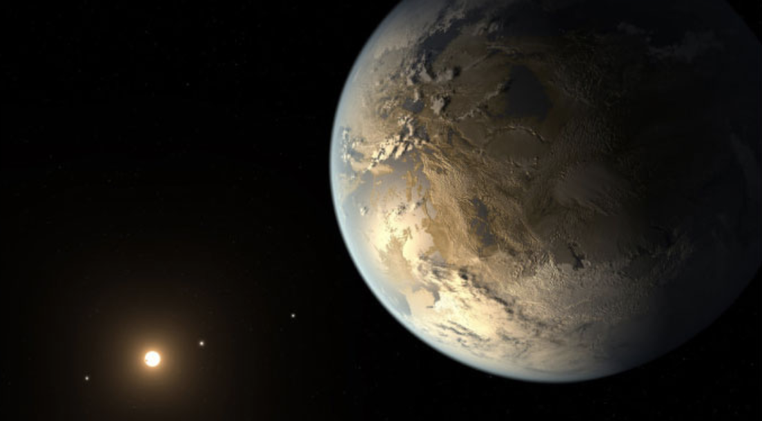
The scare-quote artist’s impression on today’s big astrobiology breakthrough seems to take its design cues from a mash-up of the stoplight-red red dwarf Gliese 581:
and the halcyon golden-hour seas of Kepler 186-f:
The best part of the article, however, is the apparently unironic use of the, “I’m not saying it was aliens … but …” construction:
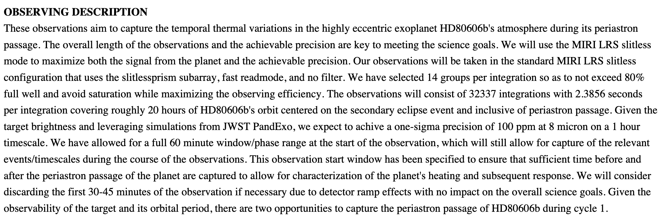
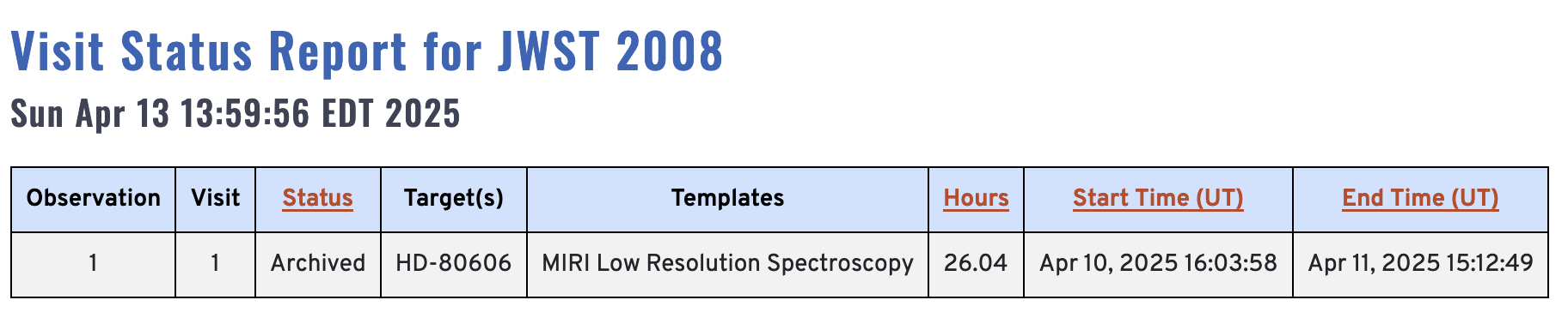
During this most recent ‘606 day, JWST observed HD80606 for 21 hours using the MIRI instrument.
Looking at the archive, it appears that the program was successfully completed.
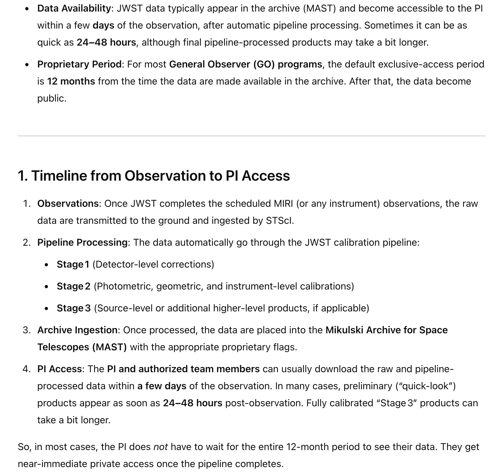
I asked ChatGPT for a run-down regarding the steps taken by the JWST science operations to process and calibrate the raw data to produce files accessible by the P.I. of the observations:
This was sufficient to rouse me in to action, flooded with nostalgia for those good old days, but with a certain steely-eyed cynicism that comes from decades spent on repeated never-quite-definitive quests to extract signal from noise. The world is non-Gaussian.
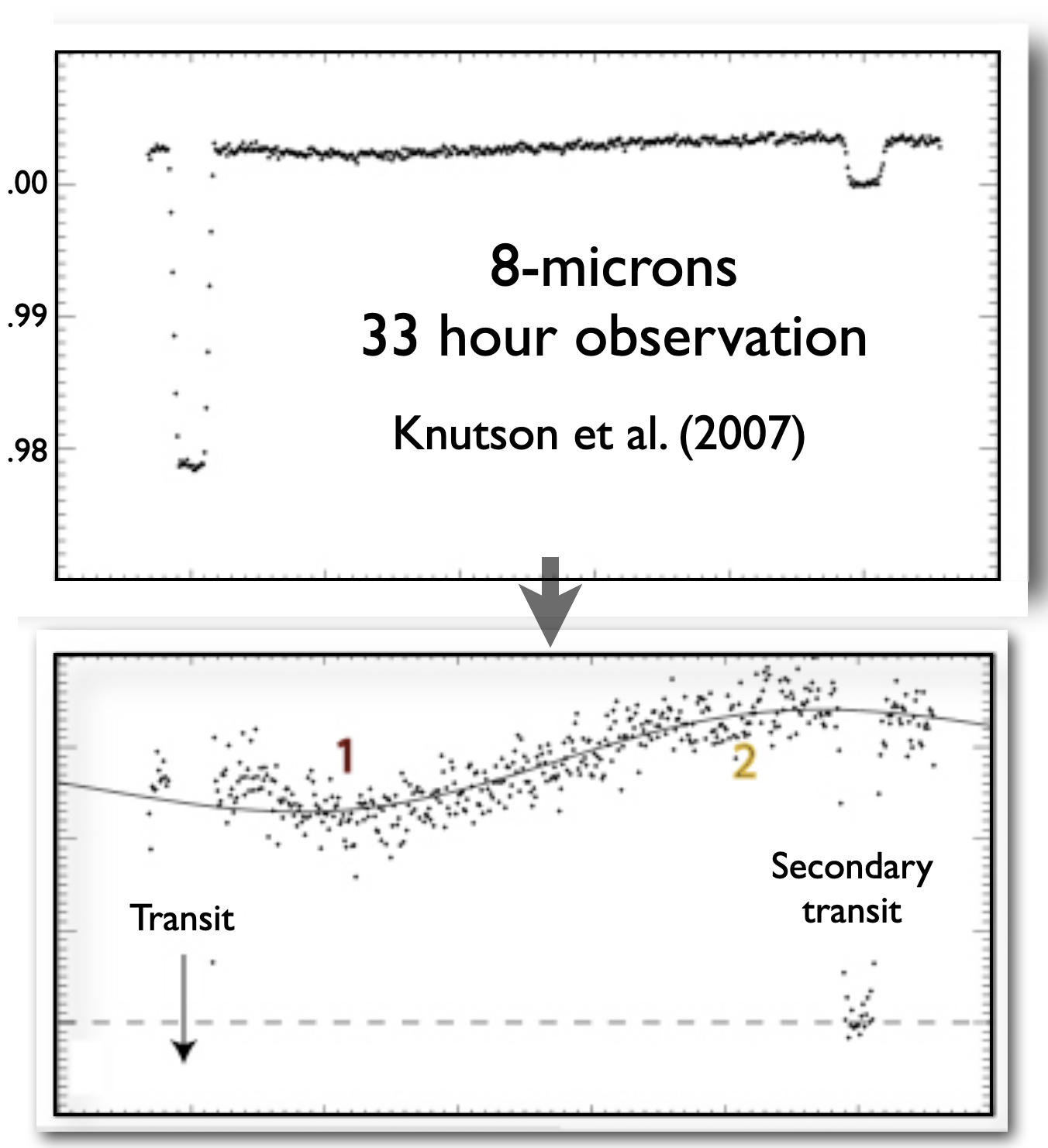
HD 80606b may be unique in that it’s a Y2K-vintage planet that’s still weird enough to be observed by JWST in a long-duration manner to produce a photometric time-series that can be directly compared with the old observations that were obtained by NASA’s Spitzer Infrared Observatory. I’m beginning to think that this might be quite a significant deal. Consider the iconic Spitzer run-down of HD 187133:
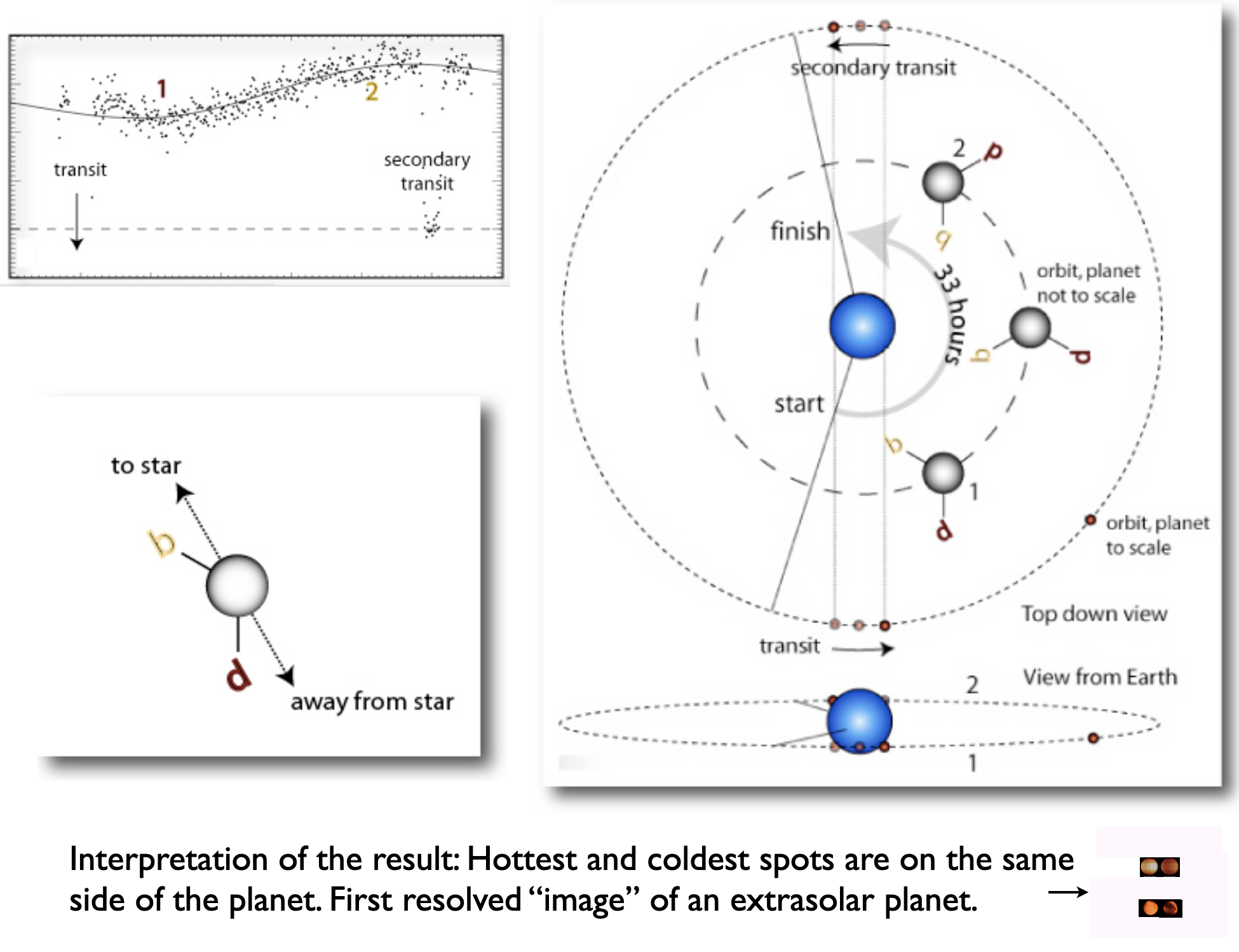
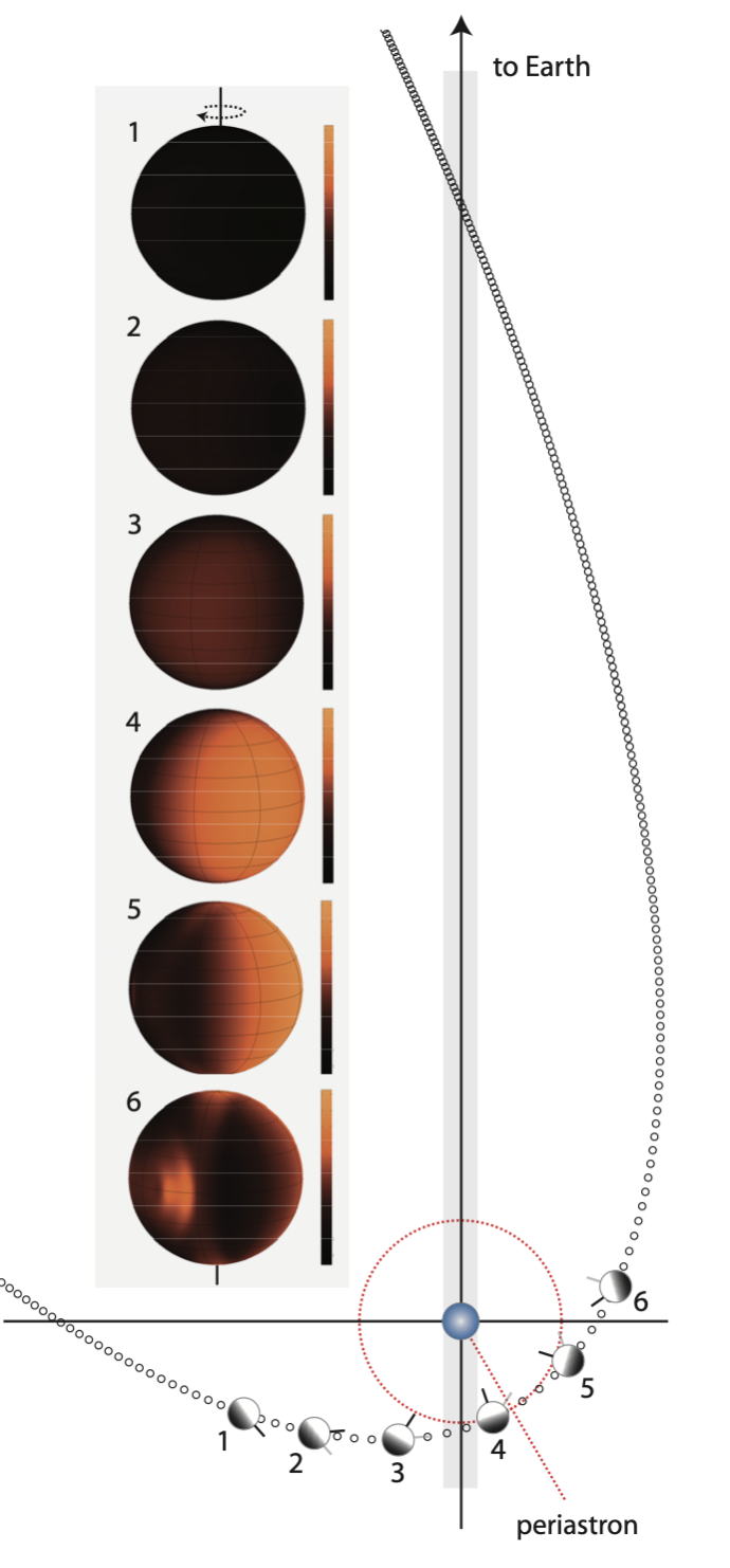
The geometry of the observation and the interpretation for what the planet was doing was as follows. Note that this assumes synchronous rotation holds:
Look at the spike in the photometry that immediately follows the transit. What’s going on there? Must be systematics stemming from the detection ramp. But, then, how do we know that the systematics are isolated to that one odd feature in the light curve? We don’t know.
The Spitzer full-phase photometric curves are rife with systematics. It’s a problem that has never been fully addressed. Where the extrasolar planets are concerned, interpretation has always run out way ahead of the data.
Coincidentally, a new paper on JWST observations of HD187133 was just published. The narrative jumps straight to the maps of the planet, with the goal of improving on those low-resolution thumbnails in the lower-right hand corner of the panel above. The full phase curve — which for Spitzer was certainly impacted by systematics — is not being observed by JWST. As a consequence, it’s unclear whether the remarkable Spitzer data can be replicated (and at what S/N) and moreover, if one looks at the lists of approved proposals, there are many many .pdfs that outline observations that push the optimistic limits.
In contrast to the situation with HD 189733, the first General Observing Cycle for JWST contained two independent HD 80606 programs that replicate long-duration Spitzer campaigns. These two JWST observational programs very similar in spirit. The first obtained a bit less than a day of continuous spectrophotometric data of the events surrounding periastron passage in the 3.8-5.2 micron band. The second (tied to that ‘606 day campaign that wrapped up yesterday) does essentially the same thing at 7-9 microns.
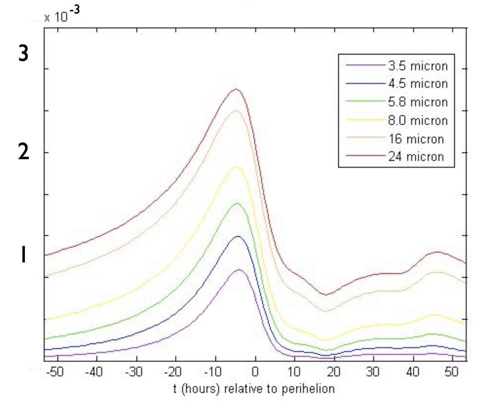
I looked back through my notes from 2007 and found some simulation results that were used to justify the original HD 80606 long-duration photometry sequence obtained by Spitzer during the cryogenic phase of its mission. We used a 2D-hydrodynamics scheme to compute what the emission from the planet should look like at Spitzer’s five photometric bands, and came up with the following then-best-effort diagram:
The resurgence in flux at 45 hours stems from the sun-blasted hemisphere of the planet pseudo-synchronously rotating back into view. The curves rely on exo-planetary properties that had never been measured, so they were necessarily uncertain. Bottom line, it was effectively fishing expedition, as nothing like HD 80606b had ever been observed.
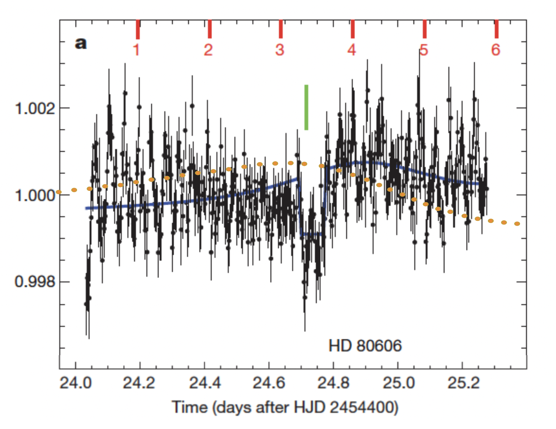
Moreover, at the time of the proposal, HD 80606’s orbital inclination to the plane of the sky wasn’t known. There was a 15% a-priori chance that a secondary eclipse would occur, and we got lucky. It did occur. Placing the yellow 8-micron prediction on the actual data gives this diagram:
The light curve can be compared with the geometry of the encounter:
The exciting result was that the planet clearly undergoes secondary transit. The disappearance of flux when the planet was behind the star unambiguously demonstrates that the photometric light curve is not all just systematics (although if one looks at it closely, systematic trends are likely present — notice how the flux seems to steadily decline prior to the start of the secondary eclipse).
Once we were in possession of the observations, the parameter deck for the hydrodynamics code could be duly and systematically varied, and a model simulation was found that provided a fit to the data. This is the blue line that runs through the photometry. We discovered that the key to getting a plausible match to the planet’s measured light curve is to adopt a short radiative timescale at the 8-micron photosphere. In keeping with widespread practice, the parameter choices that guided the simulations that supported the observing proposal were not extensively discussed in the resulting paper. If one had it to do over, it’d be better to ensure that the initial prediction and the initially predicted S/N were prominently highlighted in the article. What we got displayed a very interesting divergence from what we’d naively expected.
And in fact, now that I have a certain distance from the field, I would argue that there has never been a significant a-priori theoretical prediction in the exoplanet field that proved to be substantially correct. Hot Jupiters? Peas-in-the-pods? Radius Inflation? Ubiquitous Super-Earths? Something needs to be done to start improving on the abysmal track record…