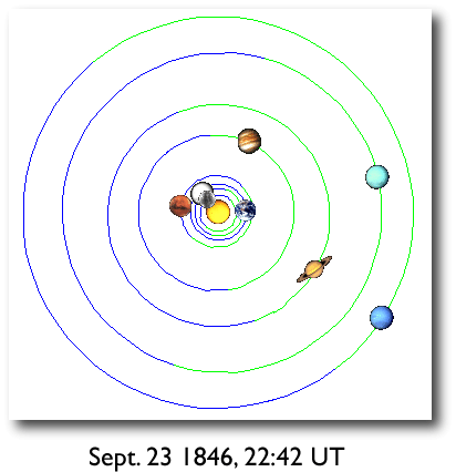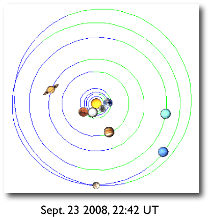
Image Source
Discoveries relating to transiting extrasolar planets often make the news. This is in keeping both with the wide public interest in extrasolar planets, as well as the effectiveness of the media-relations arms of the agencies, organizations, and universities that facilitate research on planets. I therefore think that funding support for research into extrasolar planets in general, and transiting planets in particular, is likely to be maintained, even in the face of budget cuts in other areas of astronomy and physics. There’s an article in Saturday’s New York Times which talks about impending layoffs at Fermilab, where the yearly budget has just been cut from $342 million to $320 million. It’s often not easy to evaluate how much a particular scientific result is “worth” in terms of a dollar price tag paid by the public, and Sean Carroll over at Cosmic Variance has a good post on this topic.
For the past two years, the comments sections for my oklo.org posts have presented a rather staid, low-traffic forum of discussion. That suddenly changed with Thursday’s post. The discussion suddenly heated up, with some of the readers suggesting that the CoRoT press releases are hyped up in relation to the importance of their underlying scientific announcements.
How much, actually, do transit discoveries cost? Overall, of order a billion dollars has been committed to transit detection, with most of this money going to CoRoT and Kepler. If we ignore the two spacecraft and look at the planets found to date, then this sum drops to something like 25 million dollars. (Feel free to weigh in with your own estimate and your pricing logic if you think this is off base.)
The relative value of a transit depends on a number of factors. After some revisions and typos (see comment section for this post) I’m suggesting the following valuation formula for the cost, C, of a transit:
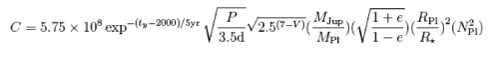
The terms here are slightly subjective, but I think that the overall multiplicative effect comes pretty close to the truth.
The normalization factor of 580 million out front allows the total value of transits discovered to date to sum to 25 million dollars. The exponential term gives weight to early discoveries. It’s a simple fact that were HD 209458 b discovered today, nobody would party like its 1999 — I’ve accounted for this with an e-folding time of 5 years in the valuation.
Bright transits are better. Each magnitude in V means a factor of 2.5x more photons. My initial inclination was to make transit value proportional to stellar flux (and I still think this is a reasonable metric). The effect on the dimmer stars, though was simply overwhelming. Of order 6 million dollars worth of HST time was spent to find the SWEEPS transits, and with transit value proportional to stellar flux, this assigned a value of two dollars to SWEEPS-11. That seems a little harsh. Also, noise goes as root N.
Longer period transits are much harder to detect, and hence more valuable. Pushing into the habitable zone also seems like the direction that people are interested in going, and so I’ve assigned value in proportion to the square root of the orbital period. (One could alternately drop the square root.)
Eccentricity is a good thing. Planets on eccentric orbits can’t be stuck in synchronous rotation, and so their atmospheric dynamics, and the opportunities they present for interesting follow-up studies make them worth more when they transit.
Less massive planets are certainly better. I’ve assigned value in inverse proportion to mass.
Finally, small stars are better. A small star means a larger transit depth for a planet of given size, which is undeniably valuable. I’ve assigned value in proportion to transit depth, and I’ve also added a term, Np^2, that accounts for the fact that a transiting planet in a multiple-planet system is much sought-after. Np is the number of known planets in the system. Here are the results:
| Planet |
Value |
| CoRoT-Exo-1 b |
$86,472 |
| CoRoT-Exo-2 b |
$53,274 |
| Gliese 436 b |
$4,356,408 |
| HAT-P-1 b |
$969,483 |
| HAT-P-2 b |
$85,507 |
| HAT-P-3 b |
$285,768 |
| HAT-P-4 b |
$189,636 |
| HAT-P-5 b |
$146,178 |
| HAT-P-6 b |
$245,873 |
| HD 149026 b |
$792,760 |
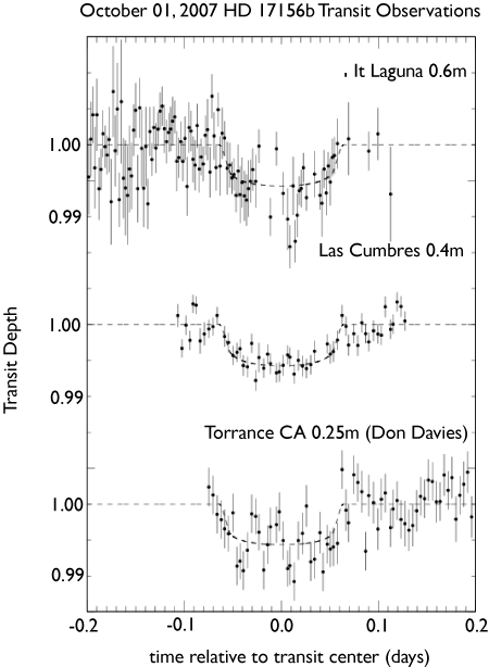
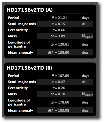
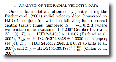
| HD 17156 b |
$953,665 |
| HD 189733 b |
$2,665,371 |
| HD 209458 b |
$11,084,661 |
| Lupus TR 3 b |
$19,186 |
| OGLE TR 10 b |
$66,112 |
| OGLE TR 111 b |
$81,761 |
| OGLE TR 113 b |
$40,153 |
| OGLE TR 132 b |
$13,523 |
| OGLE TR 182 b |
$16,743 |
| OGLE TR 211 b |
$20,465 |
| OGLE TR 56 b |
$21,680 |
| SWEEPS 04 |
$2,004 |
| SWEEPS 11 |
$211 |
| TrES-1 |
$610,330 |
| TrES-2 |
$124,021 |
| TrES-3 |
$102,051 |
| TrES-4 |
$225,464 |
| WASP-1 |
$209,041 |
| WASP-2 |
$207,305 |
| WASP-3 |
$115,508 |
| WASP-4 |
$114,737 |
| WASP-5 |
$72,328 |
| XO-1 |
$478,924 |
| XO-2 |
$506,778 |
| XO-3 |
$36,607 |
HD 209458 b is the big winner, as well it should be. The discovery papers for this planet are scoring hundreds of citations per year. It essentially launched the whole field. The STIS lightcurve is an absolute classic. Also highly valued are Gliese 436b, and HD 189733b. No arguing with those calls.
Only two planets seem obviously mispriced. Surely, it can’t be true that HAT-P-1 b is 10 times more valuable than HAT-P-2b? I’d gladly pay $85,507 for HAT-P-2b, and I’d happily sell HAT-P-1b for $969,483 and invest the proceeds in the John Deere and Apple Computer corporations.
Jocularity aside, a possible conclusion is that you should detect your transits from the ground and do your follow up from space — at least until you get down to R<2 Earth radii. At that point, I think a different formula applies.