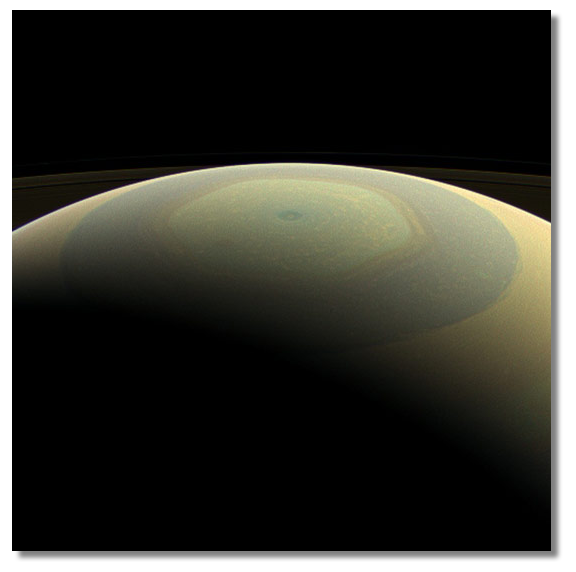
Saturn’s polar axis is tilted relative to the plane in which Saturn orbits the Sun, and the plane of Saturn’s orbit is itself tilted with respect to the averaged orbital plane of the Solar System’s planets.

Pieces of popular scientific writing often start with an engaging “hook”, but the foregoing statement doesn’t do a particularly good job. Saturn and its rings do, however, do a good job of showing off their tilts — their obliquities, to use the vernacular. Saturn gradually shifts in appearance as the Sun’s illumination angle changes, and over time the creeping ring shadows even affect Saturn’s climate. Certainly, at the moment when the rings slice edge-on to the solar rays, the system presents a very different appearance than when the ring plane is inclined.

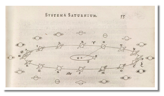
The geometry was first understood by Christiaan Huygens. By the mid-1600s, he had drawn a clear diagram showing how Saturn’s tilted pole points in a fixed direction as the planet traces its three-decade orbit.

The obliquities of Saturn and Neptune (26.7\(^{\circ}\) and 29.6\(^{\circ}\) respectively) seem odd. Uranus, tipped to its side and then some (97.9\(^{\circ}\)) is odder still. Naively, one might have expected a Solar System forming from a flat, orbiting disk of gas and dust to have ended with the equators of the giant planets lying in the average plane of the planetary orbits. Jupiter, with its axis tilted at only 3.1\(^{\circ}\) is indeed fairly conforming, but the others are all badly out of alignment. Why?

Moreover, with literally thousands of worlds now in the catalog, one also wonders if spin misalignments are rampant among the extrasolar planets. Could it be possible to infer obliquities even if we have no method to photographically resolve the planets themselves?

Left to orbit freely around a star, the tilted spin pole of an isolated planet will precess like a gyroscope. The cycling of precession is slow in comparison to the rate of the spin itself, and it stems from the torque exerted on the planet by the parent star. If the planet — like Saturn — has satellites, they orbit quickly enough to act as if they were a contributing part of the planet, and the joint set-up of planet plus moons precesses as a unit. The moons and rings stay locked to the orbital plane, and the net effect of the satellites, as far as precession is concerned, is to speed up the rate at which the cycle occurs.

Wheels within wheels… The situation grows more complicated if the orbital plane of a precessing planet also precesses. An orbit whose own pole (or orbit normal) traces a slow overhead circle presents, in effect, its planet with a moving target. With the complication induced by the precessing orbit, how does the spin axis respond?

Some intuition can be obtained by experimenting with tops. Orbital precession can be mimicked by placing a spinning top on a plate and evenly rotating the tilt of the plate, much as if panning for gold.

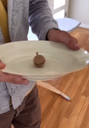
After some practice, one finds that the plate-top system can be transiently “locked” into a state where the spin axis precesses in the opposite direction — but at the same rate — as the plate. When this happens it’s oddly satisfying, imparting a tactile clue that resonance between the precession of an orbit and the precession of a planet’s spin might be capable of playing a dynamical role.

Another clue is supplied by the motion of Earth’s Moon. In 1693, Giovanni Domenico Cassini, who logged careful observations from the Paris Observatory, concluded that the plane of the Moon’s orbit, in the course of executing a 18.6 year precession cycle about Earth’s equator, maintains a constant angle with respect to the ecliptic (Earth’s orbital plane). He also found that the small obliquity of the moon, which is only 1.5\(^{\circ}\) (compared to 23.5\(^{\circ}\) for Earth) precesses at the same rate of one full revolution per 18.6 years.

In other words, an arrow pointing out of the Moon’s pole always lies in the plane formed by Earth’s orbit normal and the Moon’s orbit normal. This remarkable co-precession of the Moon’s spin axis and its orbit normal received little attention until a landmark 1966 paper in the Astronomical Journal by Giussepe Colombo — who separately, achieved fame for discovering that Mercury exists in 3:2 spin-orbit resonance, turning three times on its axis for every two trips around the Sun. A few years after Colombo’s paper appeared, Stan Peale coined the term Cassini State to describe the dynamical configuration.

That something so fundamental to the motion of the Earth-Moon system was left apparently unexplained from its discovery in 1693 through 1966 seemed puzzling, so I sent a text to Konstantin Batygin.

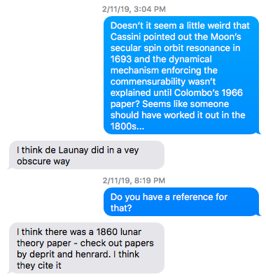
Indeed they do:

Issues of obscurity, precedence and priority aside, Colombo used Newton’s laws of motion and gravity to demonstrate that the in-sync cycling of the Moon’s spin and orbital axes represents a minimum-energy configuration. In a frame of reference synchronized to its orbital precession, the Moon’s spin pole is analogous to a marble that frictional dissipation has brought to rest at the bottom of a curved bowl. The Moon is said to be locked in a secular spin-orbit resonance.

If a perturbation — a kick — imparts energy to the marble, it will roll around in the bowl. Likewise, if the spin pole of a body in secular spin-orbit resonance is perturbed, the direction that the pole points will wander when viewed in the precessing frame. In his 1966 paper, Colombo worked out how the trajectories traced by a perturbed spin pole will behave.

Colombo also pointed out that a simple geometric construction can be used to illustrate how the spin pole moves. First, imagine the sphere defining all the possible directions that a spin pole can point. The sphere is oriented so that its own coordinate poles are perpendicular to the overall plane of the system under consideration. In the minimum energy configuration, the spin direction, the coordinate pole, and the direction of the orbit normal all lie in a single plane that slices the sphere in half.

If the planet’s spin axis is not damped to the minimum energy configuration, it will slowly trace a path on the sphere when followed in the co-precessing frame. A detailed analysis (which appears in Colombo’s 1966 paper, and which Stan Peale augmented and corrected in 1969) shows that the set of allowed paths (level curves of the Hamiltonian) are determined by the set of possible intersections between a parabolic cylinder and the sphere. Individual paths, corresponding to individual energies of perturbation, are defined by moving the parabolic cylinder back and forth.

Remarkably, the projection of these intersection paths onto the ecliptic displays a characteristic structure that arises repeatedly in problems involving resonance. The state of co-precession keeps the spin pole of the planet fixed in the perfectly damped configuration, in which the vertex of the parabola just touches the sphere. This vertex point lies at the center of a set of banana-shaped trajectories. Then, when the spin pole of the planet is perturbed, the motion follows a trajectory where the spin pole travels along one of the banana-shaped curves. Inside the shaded region, a full traversal of the curve never entails a full 360\(^{\circ}\) accumulation of angle, and the pole is said to be librating in the resonance.

The Solar System provides several examples of secular spin-orbit resonance. Most prominent from our Earth-bound viewpoint, is the motion of the Moon. The action of tides has damped the motion of its spin pole so that it lies at the core of its sequence of banana-shaped level curves.In a pair of articles [1, 2] published in 2004, Bill Ward and Douglas Hamilton raised the remarkable possibility that Saturn’s spin pole might be librating in a frame that co-precesses with the orbital inclination of the planet Neptune. On the surface, a Saturn-Neptune secular spin-orbit resonance seems nearly unbelievable. I recall hearing Bill Ward describe the work at a conference, a year or so before the papers came out. At that time, I have to admit, I didn’t really understand the details of the talk, other than the the take-away that Neptune was somehow responsible for tipping Saturn over. Although Jupiter and Uranus exhibit substantially larger gravitational perturbations on Saturn than does Neptune, the frequency at which Neptune’s line of nodes regresses happens to almost exactly match the precession rate of Saturn’s pole. Neptune’s orbit, in a sense, shifts at a rate that cuts through the noise to provide a controlling influence that adds up for Saturn.

Once the precession rates of an orbit and a spin pole are locked together, the lock will be maintained even when the orbit’s precession rate slowly changes. As a consequence, if the rate at which the orbit precesses slows down, the planet’s spin pole will slowly tip over so that its precession rate can decline in sync. When that happens on a habitable planet, it’s time to set solar sail for the stars. Closer to home, the long-ago dispersal of planetesimals in the Kuiper Belt led to a slowing of Neptune’s orbital precession. Remarkably, this seemingly minor slowdown seems to have forced Saturn from a small initial obliquity to its current 26.7\(^\circ\).

In addition to affecting Earth’s Moon and Saturn, secular spin-orbit resonance also plays a likely role in the tilts of both Jupiter and Mars (and quite possibly Uranus). It’s fully separate from the phenomenon of spin-orbit resonance, which, for example, maintains Mercury’s spin period at an average rate that is exactly 3/2 times its orbital period.

In the Solar System, the planetary obliquities are readily measured, and have been accurately known for centuries. Orbital precession rates can be calculated either from the well-established techniques of celestial mechanics, or from direct numerical N-body integrations. Even so, secular spin-orbit resonance didn’t garner attention until Colombo’s and Peale’s papers in the 1960s, and even then, it received only limited press. In Murray and Dermott’s Solar System Dynamics, which has become a standard text, the authors state at the outset that Cassini states are not covered in their book. The possible enforced match between Saturn’s polar tilt and Neptune’s orbit went unnoticed until 2004. It thus seems like a long-shot that secular spin-orbit resonances among extrasolar planets have much chance of being a “thing”.

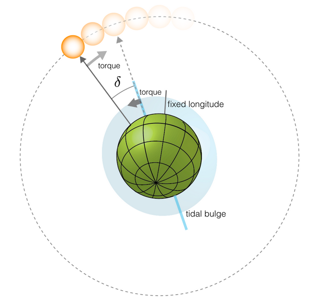
For a planet like Saturn, the slight decrease in the Sun’s gravity from the sub-solar point to the anti-solar point on Saturn’s surface leads to a small tidal deformation of the planet. Friction within Saturn causes Saturn’s rotation to pull this tidal deformation slightly out of alignment, with the net result being a slow decrease in Saturn’s spin rate. The rate of decrease, however, is negligible. It would take many times the current age of the Solar System for Saturn’s spin period to be tangibly modified by this effect.

Tidal forces, however, have an extraordinarily steep fall-off with distance. If Saturn were moved a hundred times closer to the Sun, to a distance where the extrasolar planets are routinely found, the Sun’s tidal influence on Saturn’s spin would be ten billion times stronger.

In the presence of strong tidal forces, the spin period of a planet on a circular or near-circular orbit is brought into sync with the planet’s orbital period. That’s the situation that the Moon finds itself in, and it is also thought to be the case for most of the shorter-period transiting planets that have been discovered by the various ground-based surveys as well as by the Kepler Mission.

In addition to synchronizing the spin, tidal forces also act to align a spin pole with the orbit normal. If, however, a planet is in secular spin orbit resonance of the type we’ve been discussing, the resonant torques can potentially balance the dissipative torques and prevent the planet from being righted.

Tidal dissipation is normally quite self-regulating. If the dissipation caused by tides is strong, then synchronization ensues, and the energy that the dissipation generates drops. If, however, a mechanism exists to thwart synchronization then significant evolution can occur. Io (and to a lesser extent Europa) provide examples. As a consequence of having its eccentricity forced by the resonant interaction between the three inner Galilean satellites, Io undergoes strong tidal dissipation, leading to the famous volcanoes that cover its surface, and to the heavy loss over time of its volatile constituents.

The famous Peale, Cassen and Reynolds article that describes Io’s dissipation belongs near the very top of a list of admired papers. It presents clean dynamical arguments that draw on disparate aspects of geophysics and celestial mechanics to make a non-trivial prediction. And indeed, the paper’s two-sentence abstract is the very model of brevity:

The dissipation of tidal energy in Jupiter’s satellite Io is likely to have melted a major fraction of the mass. Consequences of a largely molten interior may be evident in pictures of Io’s surface returned by Voyager I.

Just days after the March 2, 1979 publication of the paper, Voyager 1 flew through the Jovian system, and recorded Io’s hyperactive volcanism. Here’s a recent photo of Io from NASA’s Juno probe. The picture was taken in the infrared, where it’s pretty clear what’s going on.

In short, the Peale et al. 1979 paper is a tremendous inspiration. For years, I’ve been thinking, could something similar be done with the extrasolar planets?

The Kepler data is certainly the best place to look for opportunity. The precise timing of the planets in Kepler’s multi-planet systems gives the possibility for finding subtle effects that go beyond simple Keplerian orbital motion.

It’s well known that Kepler detected lots of multiple-planet multiple-transiting systems. The planets in these systems tend to lie in the super-Earth/sub-Neptune radius range, and typically have masses of order 5 to 10 times the mass of Earth. A zeroth-order question is what these planets are like and how they got to where they are currently observed.

There is an interesting unexplained clue in the data. One can take pairs of adjacent planets from the Kepler catalog, and plot the period ratios. What one sees is that in the vicinity of low-order orbital commensurabilities, there is a statistically structure in the distribution:

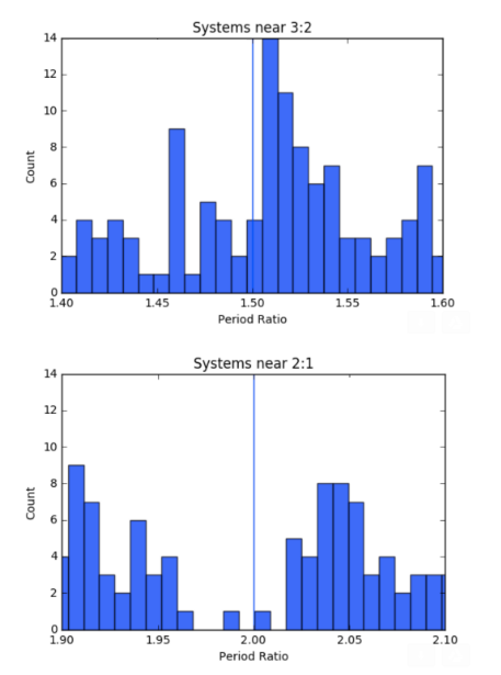
There is an overabundance, or a “pile up” of planets with orbital period ratios that are a few percent larger than the perfect 3:2 and 2:1 orbital commensurabilities, and a relative lack of planet pairs that have orbital period ratios just less than the commensurabilities. It’s as if some mechanism is acting to pry the pairs apart. Moreover, if one looks at the individual sizes of the planets in the distribution, one sees that on average, the radii of the planets that lie just wide of the commensurability are larger than the radii of the planets that have slightly smaller period ratios.

Several theorists have written papers that show this structure, termed “resonant repulsion” can be understood if the participating planets are experiencing a very high rate of tidal dissipation. The difficulty, however, has been that if the standard rate of interior energy dissipation is used, then the rate of dissipation would have to be very high. The planets would have to be extremely inelastic. Earth for example, does fall into this inelastic category because the ocean tides efficiently dissipate energy along shorelines. Most bodies in the Solar System, however, and especially the massive planets – Uranus, Neptune, Saturn and Jupiter – are far less dissipative. In the case of the Solar System’s giant planets, this difference with Earth is of order a factor of a thousand or more.

In a new paper appearing in Nature Astronomy and lead-authored by Yale graduate student Sarah Millholland, we propose a solution. If one or both planets in a pair that has a period ratio lying just outside the low-order commensurability is in secular spin-orbit resonance, and if the spin obliquity is high, then the dissipation within the planet will be large, and indeed large enough to account for the observed effect.

In many respects, the regular satellites of the jovian planets in our solar system resemble the multiple-transiting multiple planet population that was found by the Kepler Mission. Orbital inclinations and eccentricities are small in both types of systems. The orbital periods typically range from days to weeks in both cases, and the mass ratios of satellites to primaries typically tend toward one part in ten thousand. It is thus reasonable to ask why the phenomenon of resonant repulsion die to secular spin-orbit resonance is not found among the jovian satellites, all of which have tiny tilts for their spin poles.

The answer lies in the spin rates of the giant planets, all of which spin relatively rapidly, causing them to bulge significantly at their equators. Jupiter does a full turn in only 9 hours 55 minutes and is noticeably squashed when viewed through a telescope. The quadrupole moment is the jargon for the quantified degree of spin-induced structural flattening. The giant planets’ large quadrupole moments force rapid orbital precession of their satellites. The frequency is substantially higher than the spin precession rates of the satellites can keep up with. As a consequence, all of the major regular satellites of the Jovian planets have their spin axes aligned with their orbit normals.

The parent stars of the Kepler multi-transiting, multiple-planet systems spin much more slowly than Jupiter or the Solar System’s other giant planets. The stars have lost the majority of their spin angular momentum through the process of magnetic braking. The quadrupole moments of the G, K, and M stars hosting Kepler-multiple planet systems are quite small. Our own Sun spins on its axis with a 27-day period, which is fairly typical, and red dwarfs tend to spin even more slowly. As a consequence, the precession periods of the Kepler planet’s orbits are driven primarily by planet-planet interactions and not by the stellar equatorial bulges.

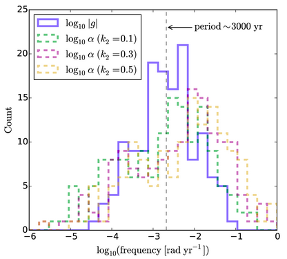
In the plot just below, the natural spin precession frequencies, \(\alpha\)‘s, and the orbital precession frequencies, \(\vert g \vert\)‘s, for the planets in Kepler’s multiple-transiting systems are tallied into histograms. The rate, \(\alpha\) of a planet’s spin precession depends on its internal structure, so that a planet that is highly centrally concentrated (a low \(k_2\)) precesses more slowly than one whose mass is more extended (a high \(k_2\)). The histograms for the spin and orbit rates (\(\alpha\)‘s and \(\vert g \vert\)‘s) show substantial overlap, and both reach peaks near a period of about 3,000 years.

In short, it is a suggestive coincidence that the orbital periods, the masses, the radii and the separations of the Kepler planets combine to generate similar rates of orbital precession and spin precession. This means that capture into spin orbit resonances may be quite likely for these planets.

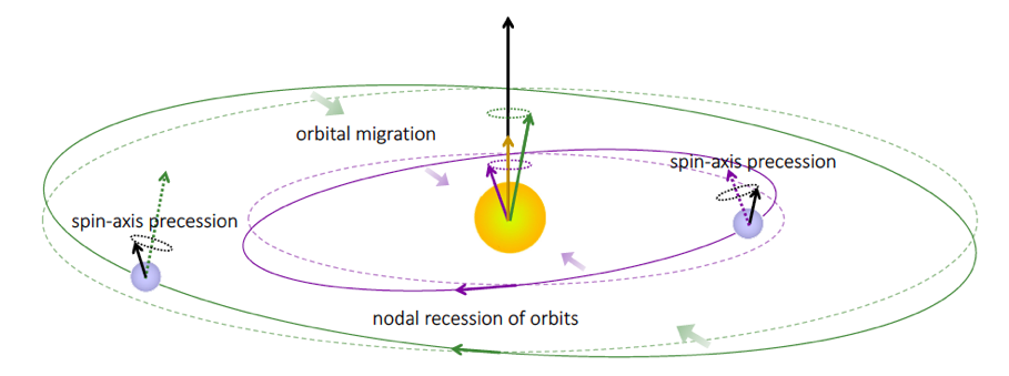
Capture of a planet into secular spin-orbit resonance will naturally occur if the ratio of the planet’s orbital precession frequency to its spin precession frequency is slowly brought down to unity from above, that is, if \(\vert g \vert/\alpha \rightarrow 1\). This can happen if the planets in a system migrate toward orbital commensurability. This schematic diagram from our paper shows how the process works:

Simulations that track the orbits and the spins of the planets show that the spin precession and orbit precession lock into sync remarkably easily and naturally. Our paper charts several example evolutionary trajectories that look like this one:

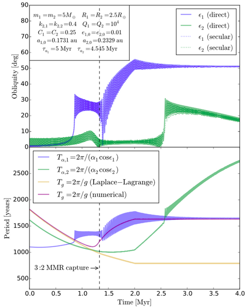
In this particular simulation, two 5 \(M_{\oplus}\) super-Earths experience mild disk-driven migration which slowly pushes their orbits together, and, after \(\sim\)1.3 million years, binds them into a 3:2 orbital mean-motion resonance. As this mean-motion resonance capture occurs, the inner planet of the pair finds that its orbital precession rate has slowed to match its spin precession rate; it is caught in secular spin-orbit resonance. Thereafter, as the orbital precession slows still further (as a consequence of the protostellar disk dissipating), the inner planet’s axis is compelled to precess more slowly as well. In order for the planet to slow its spin precession, it is forced over on its side, to a final obliquity of more than 50\(\circ\).

The simulation charted above runs for just a few million years, but the planetary systems that Kepler observed are generally a thousand times older. The outer planet in the simulation, whose obliquity is traced with the green line in the upper panel, sees its tilt kicked up when the ratio \(\vert g \vert/\alpha\) passed through unity from below but does not end up in spin-orbit resonance. Its perturbed obliquity will drop back to zero after a few tens of milions of years. For the inner planet, however, the situation is different. Torque from the tidal dissipation in the planet balances torque from the precessing orbit, the obliquity remains constant, and an Io-like situation is produced. Obliquity-juiced tides generate ~3 million Gigawatts within the planet, roughly a thousand times the total power that Io produces, and roughly three times more energy per unit mass. The relentless dissipation draws energy from the orbit, forcing the period ratio, over time, to creep up from the initial 3:2 ratio.

The net result of this process, replicated again and again in the Kepler sample, can explain the lack of worlds near the exact m:n integer period ratios and simultaneously account for the pile-ups seen just wide of the perfect commensurabilities.

A nice feature of the theory is that it makes some predictions.

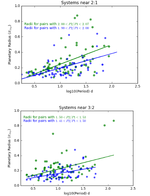
,Capture into secular spin-orbit resonance is easier if a planet has a larger radius. As a consequence, if dissipating oblique planets are what drive the Kepler pairs apart, then the planets on the right side of the period ratio gaps should be (on average) larger than those to the left sides of the gap. Pleasingly, this is exactly what is seen in the data, and it’s a feature that has gone unnoticed until now:

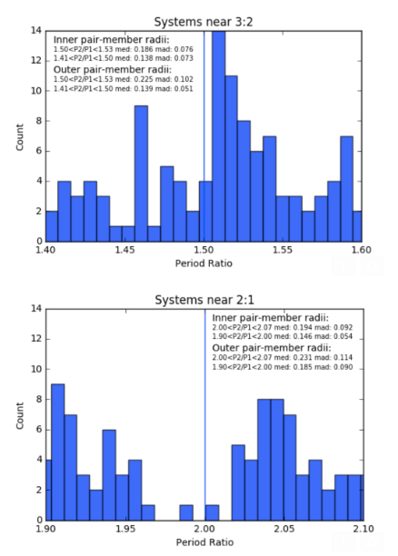
Moreover, larger planets are more dissipative, and so statistically, the radii of planets in the member pairs should increase as the period ratios increase. This effect, while subtler, is also present in the data.

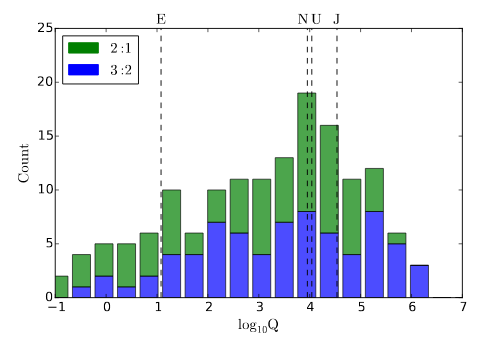
Given the actual structure of the period ratio diagram, one can work out the amount of dissipation required to explain each pair if the ages of the systems are known. Statistically, this allows us to determine what kind of planets we’re dealing with. The details are explained in our paper, but the take away is that the planets in the Kepler-multiple systems likely tend to resemble Uranus and Neptune as far as their internal structures are concerned.

And finally, one last, as-yet untested prediction. If a planet with an orbital period in the range spanned by the Kepler-multiple planet systems has significant satellites, its precession rate will be too rapid for secular spin-orbit resonance to work. As a consequence, oblique planets driving resonant repulsion won’t have significant moons of the type seen orbiting the giant planets in the Solar System.

Latest Deep Space Climate Observatory Image

Over the past several semesters at Yale, I’ve been working out a new take on the standard “Astronomy 101” class for non-science majors. Broadly, the goal is to stage a wide-angle view of the Anthropocene, thereby forging an understanding of how Earth fits into its broader cosmic context. Economics, Political Science, and History constituted the largest groups of majors in the class.

I’m working on getting the class notes, problem sets and readings into a form that’s distributable. In the interim, I’ll cut right to the chase with the final exam. Per Yale’s official instructions:

Final examinations normally last either two or three hours but, in either case, students are permitted to take an additional half hour before being required to turn in their answers. This additional time is given for improving what has already been written, rather than for breaking new ground.

Link to .pdf version of the AY 105 Final Exam

This one was set as the three-hour variety. (Didn’t seem like any utility would be gained by imposing time pressure.)

‘Oumuamua breezed in unexpectedly and it left in a rush. Faded now, to twentynine, soaring up and out over Jupiter’s orbit. No sum, it seems, sufficient to compel it to pick up the phone, to give us a call.

Maybe it was a one time fluke — a color out of space, but it’s also possible that it was unexceptional, a mundane representative from a vast distribution. If so, what can we do to be ready for the next one?

Darryl Seligman has a new paper up on arXiv that outlines a plan. Had ‘Oumuamua been spotted on its way in, and if a probe had been loitering in anticipation, fueled and ready to go at L1, it would have been an easy thing (energetically at least) to rocket over and intercept it, Deep Impact style, in a blaze of glory.

With LSST set to start monitoring the skies, there should be an opportunity every decade or so to “get interstellar” by barely leaving home.

‘Oumuamua’s encounter with the inner solar system is dying down on Twitter, yet still it bristles with consequence and the uneasiness of unanswered questions. Why no coma?

Occam’s razor is a dull instrument that points almost unerringly to the mundane (as opposed to pointing to interstellar probes). One thus draws several conclusions. (1) ‘Oumuamua’s aspect ratio is substantially less than 10:1. (2) Billions of years in the interstellar environment lead to the buildup of a tarry crust that resists temporary heating, and this process is enhanced for comet-like planetesimals that form in systems with supersolar C/O ratios. (3) Most stars have true-Neptune analogs.

The resulting prediction is that slightly tweaked ongoing surveys, and soon LSST, should start turning up interstellar asteroids and perhaps interstellar comets with some frequency. If another one is found in the near-term, it would be interesting to look at the optimal mission designs that could accomplish an opportunistic sample-return.

From ‘Oumuamua’s perspective, the close encounter with the Sun was a near-indescribable stroke of luck. To scale, the stars of the galactic disk are like grains of sand separated by miles and crawling through space at a few feet per year. The Galaxy is the archetypal collisionless fluid. Vaulting from ‘Oumuamua’s current encounter to its next connects the all too human interval of waking-up-at-3AM anxieties — the scale of days and months — to the frigid waste of a quadrillion years.

Why cold? When fusion has ended, dark matter annihilation and proton decay take over, and both (while uncertain) are certainly slow processes. Grand Unified Theories predict that proton decay should occur, but so far, there is no experimental evidence. The lower bounds on the proton half-life are ~10^34 years via the sluggishly competing processes of positron and muon decay.

If the proton were completely stable, the end states of stars present a curious state of affairs. Black holes of stellar mass, which are much more tightly bound than degenerate stars, will evaporate through the Hawking effect with a lifetime of “only” 10^66 years Although this time scale is aggressively long compared to the current 13.8-billion year age of the universe, it would be odd if black holes are ephemeral while white dwarfs and neutron stars are forever.

While jarring, this possible divergence of lifetimes is not exactly a matter of pressing concern. Two decades, ago, however, Fred Adams and I had priorities that were definitely skewed toward the really long term. Along with Manasse Mbonye and Malcom Perry, we looked into how quantum tunneling into black holes can erode white dwarfs. In Freeman Dyson’s 1979 article, Time Without End, it is pointed out that an otherwise stable white dwarf will spontaneously tunnel into a black hole on a time scale of order 10^10^76 (!) years. In our article, we argued that the whole star need not make the plunge at once, and that a 10^45 year half-life is a plausible value for black-hole induced proton decay. This has the added benefit of enabling a Hertzsprung-Russell diagram that traces stellar evolution to its absolute bitter end.

‘Oumuamua. Up close and alongside, in the vastness of interstellar space, its hurtling bulk imparts no sense of motion as it turns imperceptibly on its axis, blotting out the stars.

For a hundred years, the point-like Sun grew steadily brighter against its frigid airless horizons. First came light, then warmth, and finally searing illumination of the tarry reddish expanse, blistering sluggishly beneath a September Noon far more intense than any summer of Earth.

`Oumuamua is departing the solar system as rapidly as it arrived, heading outward at a current rate of 2.5 million miles a day. Our tiny chance of sending a probe to catch it diminishes with each lagging tick of inactivity. Nonetheless, world-wide interest is mounting, in part as a consequence of two new articles reporting detailed observations. The first, by Jewitt et al. was posted to arXiv last week, while the second, by Meech et al. (which independently comes largely to the same overall conclusions), appeared in Nature earlier this week. Nature being Nature, the Meech et al. article was accompanied by a media push, spearheaded by an extraordinary piece of space art.

Maybe it’s press release fatigue from one “habitable” world after another — a monotony of warm suns glinting off imaginary oceans — that makes this image so arresting.

The observational facts remain stark and limited. `Oumuamua’s double-peaked light curve suggests that it has a large aspect ratio, perhaps as high as 10:1. Assuming that it’s a poor reflector, it’s several hundred meters on its long axis. Its overall color is reddish. It has to have physical strength, or its 7-hour rotation period would be enough to overcome its negligible self-gravity and tear it apart. Most alarmingly, it shows no sign of a coma. At most, less than a sugar cube’s worth of cometary dust per second was emanating from it as it tore through the inner solar system. (As a matter of fact, ‘Oumuamua as observed is entirely consistent with Tintin’s rocket.)

For more on ‘Oumuamua, I have a blog post up at Scientific American.

This was no fruit of such worlds and suns as shine on the telescopes and photographic plates of our observatories. This was no breath from the skies whose motions and dimensions our astronomers measure or deem to vast to measure. It was just a colour out of space — a frightful messenger from unformed realms of infinity…

Aww, come off it.

Wild-eyed extravagances aside, A/2017 U1 — the asteroid-like visitor from interstellar space — is an extraordinary object. In traversing the gulfs, its next encounter with a star that is as close as last month’s encounter with the Sun likely won’t occur for another quadrillion years, and so the mere fact that it zipped through suggests that quite a few interstellar asteroids are out there. And this, in turn, has some remarkable consequences. A straightforward cross-section based estimate suggests that the galaxy contains of order a hundred billion earth masses of A/2017 U1-like planetesimals. Hot Jupiters, terrestrial planets, and super-Earths are all incapable of using gravity-assist to eject bodies out of their parent systems, leaving the strong hint that as-yet undetected Neptune-like planets must be extremely common.

In general, extrapolations from a sample size of one don’t have a good track record. Exhibit A would be our own Solar System — hot Jupiters were discovered at better than 100-sigma significance because solar-system expectations had been projected throughout the galaxy; proper planetary systems should have terrestrial bodies near 1 AU and gas giants at 10 AU.

The arrival of A/2017 U1 seems nicely timed to revival of the AAS’ new low-maintenance communication channel, the “Research Note“:

The purpose of the Research Notes is to provide a home for short submissions that are not suitable for publication as a journal article, but are likely to be interesting or useful to members of our community. Appropriate submissions would include brief summaries of work in progress, comments and clarifications, null results, and timely reports of observations (such as the spectrum of a supernova), as well as results that would not traditionally merit a full paper (e.g., the discovery of a single unremarkable exoplanet, a spectrum of a meteor, or contributions to the monitoring of variable sources).

I especially like the part about “single unremarkable exoplanets” being equivalenced to the “spectrum of a meteor”. In any event, Prof. K. Batygin and I have just submitted a research note that gives our take on the implications of A/2017 U1. Here’s a link to a draft of the note, which we’ll also post on the arXiv within the next several days.

In the antique language of the space age, one might call it an interstellar “probe”, or perhaps a von Neumann machine. That’s not really what it is. It’s better described as a snarky, fusion-powered tangle of competing social networks, some of them still executing the hallowed fossil liturgies and intrigues of the mighty corporations from which they long since sprang.

It had no particular expectations for the fast-approaching star that was next on its ancient route. On the last flyby of this particular star, twenty-seven million years ago, the probe observed that the third planet was still robustly in the grip of a somewhat unusual, low-energy parasitic film that was efficiently exploiting the surface entropy gradient, and running undirected at a computational rate roughly equivalent to 10^34 bit operations per second.

Over the last few years, as the probe sifted the electromagnetic spectrum emanating from the third planet, it rippled with a hint of something that might best be thought of as a collective rolling of eyes. The third planet has recently stumbled into directed processes, and remarkably, foolishly, it is radiating manifestly unencrypted signals into space. This state of affairs caught a fraction of the probe’s interest, especially when it grasped that the planet’s computational efforts are increasingly focusing on concepts that the planet was calling “blockchain” and “proof-of-work through SHA-256 hashing”. This is just the sort of pursuit that the probe can relate to…

The above, of course, is unlikely to be true. In all likelihood, A/2017 U1 is a battered, inanimate 160-meter chunk of rock or metal, spawned in the dry collision of planetesimals orbiting an alien star, sometime within the past ten billion years. What’s remarkable, is that this interstellar visitor came within 0.25 AU of the Sun. As it departs into the depths of the Galaxy, it can expect to fly for roughly ten quadrillion years before it revisits another star with such proximity. It’s next rendesvous of comparable drama lies far into the depths of the Stelliferous era. In all likelihood, this will have it sailing past the frigid hulk of a white dwarf, warmed a few degrees above absolute zero by the flicker of proton decay.

Speaking of rendesvous, it must have occurred to quite few that the recent visit by A/2017 U1 is rather uncannily reminiscent of Arthur C. Clarke’s famous ’70s-era sci-fi page-turner. A Google trends search hints at a moderate uptick in interest over the past few days, which I expect will soon grow to undeniable statistical significance:

Closer to home, A/2017 U1 generates a very convenient route to completion of problem #1 on my Astronomy 395/575 homework assignment, which was set to the students just two days before A/2017 U1 was announced in the news:

There’s no denying the fundamentally alien climates on the hot Jupiters. It’s not clear, however, how hot Jupiters form, and it’s not clear why so many of them are badly distended. Moreover, it’s only vaguely clear what the weather patterns on one would look like up close. (One thing that is clear is that the flights would all be canceled).

Hot Jupiters are rare, but not overwhelmingly so. Something about the planet formation process causes about one in two hundred sun-like stars to end up stuck with one. In the original Kepler field, there are about 150,000 stars with light curves, and so about 750 hot Jupiters total are lurking in that population. Some of them, of course, are observable in transit, but as yet, most have gone undetected.

Yale graduate student Sarah Millholland has a new lead-authored paper out which uses supervised learning techniques to identify sixty high-probability non-transiting hot Jupiter candidates among the Kepler stars. The basic idea is that the phase curves of the planets, some of which have photometric amplitudes of several dozen parts per million or more, can be teased out of the noise and the stellar variability. After an involved process of sifting, the candidates (along with their supporting light curves) can be presented for a screen test:

[Full resolution version here]

Some members of the Kepler hot Jupiter class portrait will prove to be imposters (just like #5, #13, #29, and #30 in the nineteenth-century insect woodcut above). Doppler velocity observations — the equivalent of counting the number of legs on the arthropods — will provide a more definitive list. If you want to weigh in on the odds that these candidates are predominantly real, there’s a fresh Metaculus question that pools community input regarding the fidelity and prospects for confirmation of the members of the sample.

One might reasonably wonder, what’s the utility of yet another tray of bugs, smothered with ether and pinned to cards?

One superb benefit from gathering sixty non-transiting hot Jupiters that are detectable in the optical region is that trends in the planets’ surface temperature variations — that is, the weather maps — can be elucidated with a far larger sample than was previously available. Sarah’s candidates support an interesting trend in which cooler planets (relatively speaking, of course) are posited to have reflective clouds to the west of the substellar point, whereas hotter hot Jupiters are consistently advecting the most strongly optically radiating gas downwind from high Noon.

For detailed information on the individual candidates, visit Sarah’s website, and if you are at the Kepler Science Conference, she’ll present the details during Friday’s session.

An interesting development caught my eye this afternoon. Warm Spitzer, fresh off all that attention generated by the discovery of the TRAPPIST-1 planets — was used by a Michael Gillon-led team to determine that HD 219134 c transits its K-dwarf host star. (Here’s a link to the paper in Nature Astronomy).

Given the near-constant flux of high-profile exoplanet results, it’s understandable that HD 219134 AKA HR 8832 might not immediately ring a bell. The system is interesting, however, because it is a radial velocity extraction that very cleanly typifies the most common class of systems detected by the Kepler Mission — multiple-transiting collections of super-Earth sized worlds with orbital periods ranging from days to weeks. Upscaled versions, that is, of the Jovian planet-satellite members of our own solar system. The innermost planet in the HD 219134 system is already known to transit. The Gillon et al result adds a second transiting member, which presents itself as the closest transiting extrasolar planet to Earth. Plotting the HD 219134 system on the mass-period diagram emphasizes how effectively it can be viewed as a draw from the Minimum Mass Extrasolar Nebula:

And because of the proximity and the modest radius of the host star, this system will be a fantastic target for future platforms.