Lone Star

Frequent visitors to oklo.org will have noticed that the new posts have dried up over the past several days. I was out of town to attend the 2nd annual Mitchell Institute Symposium at Texas A&M. This is a conference that brings together speakers from a broad range of sub-disciplines in Astronomy and Physics. Ten gallon hats off to Texas! I had a great time. Warm weather, informative talks, and the Aggies all called me “Sir”. My plan for next week is to get the UCSC Banana Slugs to start up with that tradition.

As part of the conference, I was asked to give a public talk on Extrasolar Planets. It was an all-day scramble on the laptop to get all my slides together into a coherent whole, but the talk ended up being a lot of fun. The audience was highly informed and engaged. The TAMU Physics Department definitely got the word out. I was completely stunned this morning to find that I was on the the front page of the Bryan-College Station Eagle, and I was even recognized at the College Station Airport cafe while I was waiting for my flight out. Unbelievable.

Here’s a link to a quick-time movie, as well as a .pdf file with the slides that I showed during the talk. I’ve also put the sound files (you had to be there to know what I’m talking about) here, here, and here in .wav format. A future oklo post will go into much more detail about what’s being heard in these files, and how they are generated.

If you’re new to the site, here’s a bit of information. Oklo.org is the home base for the systemic collaboration, which is a public participation research project aimed at obtaining a better characterization and understanding of extrasolar planets. Everyone is invited to participate, and details and updates are given regularly in our systemic faq posts.

We have been developing both the oklo.org site, as well as the systemic console using a Mac OS-X platform. We have been testing both the site and the console using Internet Explorer, and we have gotten generally good results, but it is clear that some users are experiencing problems. We are working hard to clear these issues up. We’re astronomers by trade, and, and sadly, at the moment, it’s strictly amateur hour when it comes to website development. As an example, you should see a menu of links directly to your right. I recently saw the oklo.org site on a Windows-IE combination in which the links had been mysteriously pushed all the way down to the bottom of the page. I had to scroll all the way down to even see them.

Also, if you are a Macintosh user, run the console in Safari. There is a still a Java issue with the Firefox on OS X. Firefox should, however, work fine on both Linux and Windows machines if your Java libraries are up to date…

Give us a place to stand

In early June of 2001, I was sitting at my desk at the NASA Ames Research Center trying to debug a computer simulation. Outside my window, the traffic was gridlocked on Highway 101. The distant folds of the Diablo Range shimmered in the California Sun. The phone rang, jarring me out of my abstracted state of mind.

yucca

“Dr. Laughlin? Its Robin McKie of the London Observer.”

His voice seemed friendly and reasonable, and I’ll admit that I was pleased to have warranted a call from an overseas reporter. To the best of my recollection, our conversation started something like this:

“Well the reason I’m calling is because I recently saw an abstract of your work concerning this so-called idea of `Astronomical Engineering’, and I was wondering if you could take a few minutes to fill me in on what its all about?’’

(more…)

Some evidence for the existence of 51 Peg c

This post continues with a thread that we’ve been developing over the past several days (posts 1, 2, and 3). In brief, we’ve found interesting evidence of a second planetary companion to 51 Peg in the published radial velocity data sets.

a single spike in a periodogram

We first used the Systemic Console to recover 51 Peg’s famous (P=4.231 d) companion from the data, and then looked at the power spectrum of the residuals to the single planet fit:

residuals

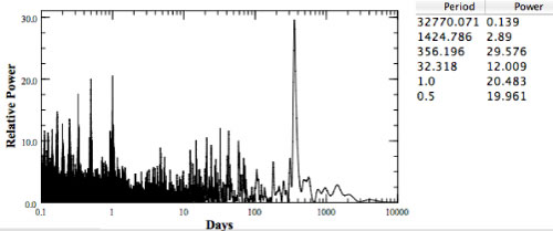
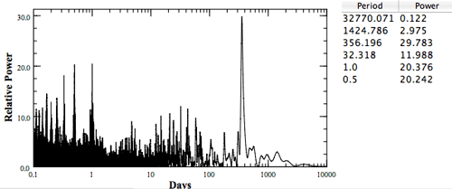
There is a startlingly large periodicity in the data at a 356.2 day period.

We then used the console to identify this periodicity with an Msin(i)= 0.32 Jupiter-mass planet in an e=0.36, P=357 day orbit.

There’s no question that the addition of this second planet reduces the scatter in the data relative to the model. The question is: can the model be taken seriously? Is 51 Peg “c” really there?

(more…)

51 Peg c

In the posts for Thursday and Friday, we used the Systemic Console to explore the radial velocity variations of 51 Peg. Aside from harboring the first extrasolar planet discovered in orbit around a Sun-like star, this data set is extraordinary because it contains nearly 270 individual radial velocity measurements taken over a period of over ten years. Very few stars have published data sets that are so extensive.

Get on board!

After extracting the signal of the celebrated 4.231 day planet from the data, we computed a periodogram of the residuals. The calculation shows a strong concentration of power at a 356 day periodicity:

residuals periodogram for 51 Peg

At the end of yesterday’s post, we were left hanging on the suggestion that this strong peak might represent a second planet in the 51 Peg system. Let’s have a look at this hypothesis by making a two planet fit to the data.

If you’ve gone through the systemic tutorials, and are comfortable at the controls of the console, here’s the procedure:

Launch the console and follow the directions given yesterday to obtain the best single-planet fit to the data. Next, activate a second planet, and enter 356. into the data window of the period slider for the second planet. Then, minimize the new planet’s mean anomaly, followed by a minimization on the mass. Next, send all ten orbital parameters for the two planets, along with the velocity offsets off for a polish by the Levenberg-Marquardt algorithm. Note that it’s fine to push the “polish” button several times in succession, to ensure that the algorithm has been given enough iterations to converge to the best fit in the vicinity of your choice of starting conditions.

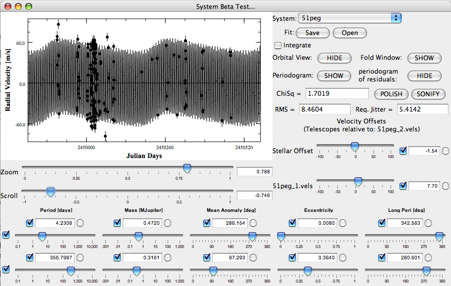
The console shows that the addition of a second planet improves the fit to the data, dropping the chi-square to 1.7, and reducing the required jitter to 5.4 m/s.

The second planet, which we’ll call 51 Peg “c” (where c stands for “console”, huh, huh) has a period of 356.8 days, a minimum mass of 0.32 jovian masses (slightly larger than Saturn), and an orbital eccentricity, e=0.36. Here’s a link to a screenshot of the console showing all the parameters. This is also an advance look at the next version of the console which Aaron will be releasing in a few weeks.

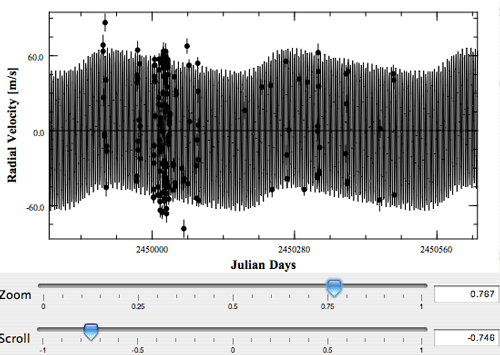
Using the console’s zooming and scrolling sliders, we can see the modulation of the radial velocity curve. The second planet imparts a visibly non-sinusoidal envelope on the strong carrier signal created by 51 Peg b. The non-sinusoidal shape stems from the significant eccentricity of planet “c”:

radial velocities response from 2 planets

Note that we still have to teach the console to draw smooth curves when the zoom level is high! Look for that improvement to show up in about 2 months or so. There’s a lot of other items ahead of it on the to-do list.

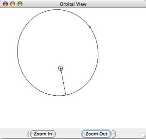
The orbits of the two planets look like this:

51 peg b and c

Does it really exist, this room-temperature Saturn? Is it really out there? Do furious anticyclonic storms spin through its cloud bands? Does it have rings? Does it loom as an enormous white crescent in the deep blue twilight sky of a habitable moon?

Maybe.

Eugenio and I have been working through the weekend to devise statistical tests which can assess the likelihood that this planet exists. We’ll check in shortly with our results

Quetzalcoatl

One evening last August (0. 12. 19. 12. 10. 10.) I was filling my car with gasoline. Venus hung low and bright above the horizon in the deep blue twilight. In the foreground stood the glowing red and yellow symbol of Shell Oil. Swirling coils of aromatic hydrocarbons dissipated in the cool marine air.

The ancient Maya were obsessed with Venus. At the times when it was visible, they covered windows and doorways to protect against its rays of mirrored sunlight.

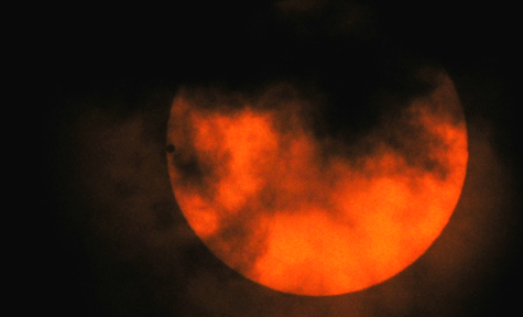
venus in transit

Venus’ brilliance in our skies arises partly because of its proximity, and partly because it is completely covered with thick white clouds that drift through the upper layers of a CO2 atmosphere roughly 100 times more massive than Earth’s. Venus, however, may not always have been so inhospitable. The high Deuterium to Hydrogen ratio in its atmosphere indicates that it has lost a lot of water. It is possible that during the first billion years of the Solar System’s history, Venus had liquid water, perhaps even an ocean, on its surface. If this was the case, then Venus shone down with less brilliant menace in the Archean skies.

In two, or perhaps three billion years from now, the Earth will have shared Venus’ fate, and will glow with pure-white intensity in the salmon twilight of the Martian evenings.

(Note: the above image of Venus in transit is a screenshot detail from a .jpg image on the website of the Venezuelan Centro de Investigaciones de Astronomia.)

51 Pegged?

Yesterday, we supplied the Systemic Console with the published radial velocity datasets of the the planetary system that started it all, the original gangsta, 51 Peg.

It’s interesting, after more than a decade of observation, to see what happens as a radial velocity time series acquires a long baseline. Launch the Systemic Console, and select 51 Peg from the system menu. You’ll see a plot that looks like this:

radial velocity data sets for 51 Peg

With the “51peg_1.vels” offset slider, it’s easy to separate the two contributing data sets. (One was published by the California-Carnegie Planet Search Team, the other by the Geneva Extrasolar Planet Survey). The Swiss data set gives a long baseline of coverage, whereas the California-Carnegie dataset contains intensive observations taken mostly over the course of a single observing season in 1996. Click on the periodogram, and be patient while the console works through the Lomb-Scargle algorithm. While you’re waiting, you can look eagerly forward to the fact that in Aaron Wolf’s next release of the console (due in a few weeks) the periodogram calculation will be sped up by more than a factor of ten.

power spectrum for 51 Peg

The periodogram has an impressive tower of power at 4.231 days. This dataset contains a whopping-strong sinusoidal signal:

To work up 51 Peg “b”, activate the first row of planetary orbital element sliders and type 4.231 into the period box. Then (1) line-minimize the mean anomaly, (2) line-minimize the mass, (3,4) line-minimize both offset sliders, and (5) line-minimize the period. (6) Activate a small eccentricity, (7) move the longitude of periastron slider off the zero point, and then (8) click the Levenberg-Marquardt boxes to the left of each entry box and polish the fit. (If this sounds like gibberish, yet also exciting, we’ve written three tutorials [here, here, and here] that go into detail regarding the use of the console. In addition, all posts marked “systemic faq” contain information about how to use and work with the console.)

When I do this, the console gives me a single planet fit with P=4.2308 days, M=0.4749 Jupiter Masses, and eccentricity e=0.014. These values are in full agreement with the orbital parameters published in the original discovery paper.

Alert readers are likely grumbling that we’ve made no mention of uncertainties in the orbital elements. This is an extremely important and interesting issue for many systems, and we’ll definitely be posting extensively on the topic and theory of computation of errors in orbital elements of extrasolar planets. The entire Systemic research collaboration, in fact, is primarily concerned with resolving the issue of how to establish confidence levels in various types of planetary system configurations.

In the meantime, however, use the console to compute a periodogram of the velocity residuals to the old-school 1-planet fit. A strong peak stands out at a period of 356.196 days. The chi-square statistic of the 1-planet fit is just over 2.00, and the required stellar jitter is about 7 meters per second. This is significantly higher than the 3-5 meters per second of long-term jitter that is expected for a quiet, old G2 IV star like 51 Peg:

residuals periodogram for 51 Peg

Could there be another planet in the system? Could it be, that the console, by virtue of the fact that it readily combines data sets from different published sources, has found a new world (in a habitable orbit no less)? Tune in tomorrow to find out…

O.G.

Most of the recent scientific papers on the general topic of extrasolar planets start with a sentence very much like this one:

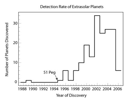
Following the announcement of the planet orbiting 51 Peg (Mayor & Queloz 1995), over 170 planets have been discovered in orbit around solar type stars.

straw

And indeed, Mayor and Queloz’s discovery of the hot Jupiter orbiting 51 Peg was truly a watershed event. Their Nature paper has racked up 764 ADS citations. Of order several billion dollars have been spent (or will shortly be spent) on the worldwide effort to locate and characterize alien solar systems. It’s thus a little weird that the Systemic Console has so far failed to include 51 Peg in its system menu. We’ve just corrected this oversight by adding the two published data sets for 51 Peg.

console selection menu

The closely spaced data near the beginning of the time series is from Marcy et al. (1997), who began intensively monitoring the planet from Lick Observatory as soon as the discovery was announced. The widely spaced data is from the Swiss planet hunting team (Naef et al. 2004), and contains 153 radial velocities obtained over a ~10-year period. The data is catalogued at CDS, and available at this link.

The 51 Peg data sets are interesting for a number of reasons. I’ll check in tomorrow with more details as to why. In the meantime, fire up the console and start finding fits.

systemic 002

There’s a new data set on the Systemic Console. To access it, launch the console, and select systemic002 from the system menu (it’s the second from the bottom of the list).

Let’s just say I’ve often wondered whether these particular data can be modeled by a stable planetary system.

Photometric Imaging

Yesterday’s post talked about how Young, Binzel and Crane (2001) used high-cadence photometric observations of Charon transiting the disk of Pluto to construct a two-color image of Pluto’s surface. Transiting extrasolar planets can be employed in a similar way to create an image of the strip of stellar surface that lies beneath the path of an occulting planetary disk. Resolution-wise, this procedure is the effective equivalent of a satellite in low-Earth orbit making a detailed image of a stripe across a sand grain sitting on the Earth’s surface.

poppies transiting a vase

In 2001, Tim Brown and his collaborators used the STIS spectrograph on Hubble Space Telescope to obtain what has become an iconic composite light curve of the HD 209458 b transit. It’s probably fair to say that the majority of talks given by astronomers on the general topic of extrasolar planets have a powerpoint slide that shows the Brown et al. data. (The astro-ph version of their article is here).

Here’s a figure (done in Adobe Illustrator, like all of the other www.oklo.org diagrams) that shows their data:

transit of HD 209458b obtained with HST

The Brown et al. light curve contains 684 time samples spaced at an average cadence of 80 seconds with a relative precision of one part in 10,000 per photometric data point. (This photometric accuracy is easily good enough to detect the transit of an Earth-sized planet across the face of a Solar-size star if one knew when and where to look.) Because HST can only observe for about half of its 96.5 minute orbit, and because the transit lasts 184.25 minutes, the light curve was obtained by stitching together photometry from groups of observations obtained on four separate transits that took place between April 25 and May 13, 2000.

An interesting feature of the above diagram is that the transit light curve does not have a flat bottom. This results from brightness variations on the surface of the star itself. Stellar disks display a phenomenon known as limb darkening. If you can resolve a star (as one effectively does when one obtains a photometric light curve of a transit) you see that the center of the stellar disk is brighter than the edges. This effect occurs because when one looks at the stellar limb, the line of sight samples higher, cooler layers of the stellar atmosphere. When one looks straight at the middle of the star, one is seeing further in, to deeper, hotter layers. For a star like the Sun or HD 209458, this effect is quite significant. The intensity at the limb is only about 40% as much as that at the center of the stellar disk. The curved bottom of the time-series, then, could be inverted and processed to construct an image of the surface of the star beneath the planet. Additionally, if the transit is observed through different color filters, then one can build a colored image of the stellar strip.

More recently, Brown and Company have made similar HST observations of the TrES-1 transit. Their light curve in this case shows a bizarre uptick, which causes the transit to resemble a one-toothed grin:

transit of TrES-1 obtained with HST

The interpretation of this feature is that the planet covered up a starspot as it traversed the face of the star. Starspots — that is, sunspots on other stars — are cooler, and hence dimmer than their surroundings. When a starspot is occulted by the planet, the fraction of blocked starlight decreases. Photometric light curves really do give us an image of a strip of the stellar surface.

For those who prefer not to shave with Ockham’s razor, there’s a second, rather more exotic interpretation of the TrES-1 transit light curve. It’s possible (although highly unlikely!) that a second, longer-period, planet was also transiting TrES-1 at the time when the uptick in the light curve was recorded, and that the inner (known) planet happened to pass underneath the outer planet, as seen from Earth. According to Tim Brown (during a talk I heard him give in Japan) this model, while crazy, does just as good a job of fitting the photometric data!

TrES-1 is an 11.8 magnitude star, and the transits are thus highly suitable for measurement by amateur astronomers using the technique of differential aperture photometry. On the transitsearch.org website, there’s an extensive discussion of amateur observations that were made in the months following the discovery of the transit by Alonso et al. Many of these amateur light curves show strange asymmetric features. It’s likely that they were also observing the planet crossing over starspots. If this was indeed the case, then the 2-planet interpretation of the “tooth” can be safely ruled out.

I should emphasize that transit observations using HST are of blockbuster-level scientific value. The exquisite HST photometry allows a very accurate measurement of the planetary radius, which in turn puts strong constraints on our theoretical models of the planetary interior (see this post for more information). The transit also strongly constrains the elements of the planetary orbit, and the color-dependence of the light curves permits the measurement of atmospheric constituents such as sodium and carbon monoxide.

The above diagram for the TrES-1 transits is adapted from a review article entitled, When Extrasolar Planets Transit their Parent Stars that I co-authored with Dave Charbonneau (Harvard University), Tim Brown (The High Altitude Observatory), and Adam Burrows (The University of Arizona). It will be published in the forthcoming Protostars and Planets V Conference Proceedings.

Here at www.oklo.org we strive to keep things on the positive tip, but I do have one disappointing piece of news to report. I was a Co-I on Tim Brown’s recent HST Cycle 15 proposal to obtain a high-precision photometric time series of the HD 149026 b transit. The resulting light curve would have had higher photometric precision than both the TrES-1 and HD 209458 b time series shown above. The light curve would have had a higher cadence, the individual points would have been good to about one part in 20,000. (At magnitude 8.16, HD 149026 is about thirty times brighter than TrES-1, and the new ACS camera on HSTT is better-suited to the photometric transit-measurements that the defunct STIS spectrograph that was used by Brown et al. for HD 209458). Unfortunately, we learned yesterday that the proposal was not accepted. This is a bummer. An HST transit light curve would have dramatically improved our characterization of the planet that has already provided the first incontrovertible evidence for the core-accretion mechanism of giant planet formation. I think that the HD 149026 light curve would likely have been as informative as the Brown et al. HD 209458 light curve, which was recently shown as #4 in the list of Hubble’s top ten scientific achievements.

The ninth planet

The frigid outer reaches of the solar system are generating a lot of activity. Pluto, Charon, Sedna, Quaoar, and 2003 UB313 all clamor for attention on the pages of the New York Times. The glamour to be gained from discovering these strange cold orbs has produced skulduggery of the highest caliber: the hacking of internet observing logs, the computation of an orbit from a series of telescope pointings, a hasty search of a guilty patch of sky. This is the stuff of thrillers. I’ve enjoyed it from the sidelines.

I have no stake and little interest in the “Is Pluto a Planet?” debate, but one point does seem clear. I seriously doubt that New Horizons would currently be on its way to the edge of the Solar System if Pluto had been stripped of it’s planetary status in 1978 when its tiny mass was finally revealed by the discovery of Charon. An unexplored outer planet can captivate the imaginations of congressional staffers. The 2nd-largest known member of Colonel Edgeworth and Dr. Kuiper’s belt just doesn’t have the same effect.

And I’d certainly pay my ~ $2.50 share to see a close-up picture of 2003 UB-313 as well…

2-color reflectivity map of pluto

Surprisingly, the image of Pluto shown above is not a photograph in the usual sense. Rather, it’s the two-color reflectivity map of Pluto’s sub-Charon surface that was obtained by (Young, Binzel & Crane 2001) with photometric transit observations. From 1985 through 1990, Charon’s orbital plane with respect to Pluto was close to alignment with the line of sight from Pluto to the Earth. This allowed a map of Pluto’s surface to be constructed by keeping careful track of the brightness of Pluto as Charon transited different chords across Pluto’s face. Measurements of the brightness through two different filters (B and V) allowed a two-color map to be produced. It’s not clear what causes the surface of Pluto to vary in reflectivity. One possibility is that we are seeing patches of methane frost.
Here’s a stop-action movie of Pluto and Neptune during the course of three Neptune orbits. Due to the 3:2 resonance between Pluto and Neptune, Pluto executes close to 2 orbits during the time it takes Neptune to go around the Sun three times. The animation was produced by integrating the two planets with a computer, and then plotting their positions at equally spaced time intervals on a sheet of paper. Peppercorns are then placed on the paper to represent the positions of Pluto and Neptune, and a Kumquat is placed at the position of the Sun. The peppercorns are then “integrated” through their motion using stop-action photography, and the resulting .jpg frames are processed into .mp4 and .mov format animation files.

frame from the pluto-neptune animation

pluto_and_neptune.mp4: If the .mp4 file won’t load in your browser, try this small version: pluto_and_neptune.mov.

two for the show

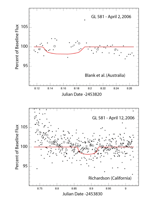
As I’m writing this, it’s about 22:08 UT, April 2, 2006. (JD 2453828.4226). The midpoint of the most recent predicted transit window for GL 581 b occurred a few hours ago, at 15:46 UT. That was in broad daylight in both the United States and Europe, but it was in the middle of the night in Australia and Japan. Hopefully, the Australian and Japanese participants in Transitsearch.org had clear weather at their observing sites.

what exactly is it?

As dicussed in previous posts, GL 581 “b” has a minimum mass of 17.8 times the Earth’s Mass (very close to the mass of Neptune), and orbits with a 5.366 day period around a nearby red-dwarf star. The a-priori geometric probability that GL 581 b can be observed in transit is 3.6%. Because the orbit of the planet has been well-characterized with the radial velocity technique, we can make good predictions of the times that transits will occur if the plane of the planet’s orbit is in close enough alignment with the line of sight to the Earth. The star can then be monitored photometrically during the transit windows to look for a telltale dimming lasting a bit more than an hour as the planet crosses the face of the star.

If GL 581 b is found to transit, then we will have a scientific bonanza on our hands. The size of the planet, and hence its transit depth, is highly dependant on the planet’s overall composition. If it is an “ice giant”, with a similar overall composition and structure to Neptune, then it should have a radius about 3.8 times larger than Earth, and it should block out about 1.7% of the star’s light at the midpoint of a central transit. If, however, the planet is a giant version of the Earth, with an iron core and a silicate mantle, then it will be considerably smaller and denser, with a radius only ~2.2 times that of the Earth. If the planet is a super-Earth, then the transit depth will be much smaller, and only about 0.6% of the star’s light will be blocked. A 0.6% transit depth is tough to detect, but it’s nevertheless possible for skilled amateur observers to reach this precision.

Here are some cutaway diagrams showing the internal structure and relative sizes of Jupiter, and of GL 581 b in each of the two possible configurations:

Core comparisons

Why would it be a big deal if we could determine the internal structure of GL 581 b? If the planet is a Super-Earth (that is, if the transit depth is small), then we would know that it accreted more or less in situ, using water-poor grains of rock and metal. The existence of such a structure would strongly suggest that habitable, Earth-like planets are very common in orbit around the lowest-mass M dwarf stars. That is, it would verify that high surface densities are a ubiquitous feature of the innermost disks of low-mass stars. On the other hand, if the planet turns out to be similar in size and composition to Neptune, then we will know that it is made mostly of water-rich material, and that it had to have accreted at a larger radius, beyond the so-called snowline of GL 581’s protoplanetary disk.

hd 20782 oct 20, 2006 (3.6%)

As advertised in yesterday’s post, three newly published radial velocity data sets have just been added to the system menu of the Systemic Console, and to the www.transitsearch.org candidates list. The data set for HD20782, published by Jones et al. of the Anglo-Australian Planet Search, is definitely the most interesting of the trio. Let’s work the HD 20782 velocities over with the console, and see what they have to say.

sunset

First, fire up the console. (If you use Firefox on Windows, and you’ve had success getting the console to work with that particular line-up, please post a response in answer to Vincent’s comment on yesterday’s post. All of Aaron’s oklo.org Java development has been done on Mac OSX using Safari. Also, we’ve had many reports that the console works well with Internet Explorer on Windows, so if Firefox won’t run the Java, give IE a try. And could someone ask Mr. Bill G. to send me a check for that plug?)

At any rate, the HD 20782 radial velocity data set has one data point that sticks down like a sore thumb:

velocities

Activation of one planet and a little bit of fooling around with circular orbits shows that even when the discrepant point is ignored, the waveform of the planet is not at all sinusoidal. The points contain an almost sawtooth-like progression:

circular orbit fit

Because of the non-sinusoidal nature of the velocities, the periodogram (obtained by clicking the periodogram button) is rather uninformative. There’s a lot of power in a lot of different peaks, and it’s not immediately clear what is going on planet-wise:

periodogram

Aaron has been working very hard on console development, and we will soon release an updated version with a number of absolutely bling features. Ever wondered what your fits sound like? One new feature is a “folding window”, which allows the data to be phased at whatever period one likes. The folding window is very useful for data-sets of the type produced by HD 20782. It quickly reveals that something like a 600 day periodicity brings out the overall shape of the planetary waveform:

folding window

Using 600 days as the basis for a 1-planet fit, activating eccentricity, and using a combination of slider work, 1-d minimization, and Levenberg-Marquardt, eventually produces excellent fits to the data that look like this:

fit to hd20872

Jones et al., for example, in their discovery paper, report an orbital period of P=585.86 days, an eccentricity, e=0.92, a mass (times the sine of the unknown orbital inclination) of Msin(i)=1.8 Jupiter masses, and a longitude of periastron of 147 degrees.

This planet is one bizzare world, and seems to be very similar to HD 80606 b (another oklo.org favorite). The orbital period is 1.6 years. The planet spends most of it’s time out at ~2.6 AU. In our solar system, this distance is out beyond Mars in the inner asteroid belt. Once per orbit, however, HD 20782 b comes swinging in for a steamy encounter with the star. The periastron distance is a scant 0.11 AU, roughly half Mercury’s distance from the Sun. The planet is likely swathed in turbulent white water clouds. Raindrops vaporize as the star looms larger and larger in the sky.

Stars that loom large in alien skies are good news for transitsearch.org, and in the case of HD 20782 b, we here on earth are particularly fortunate. HD 20782 b’s line of apsides lies within about 60 degrees of alignment with the line of sight to the Earth. This raises the a-priori geometric probability of having a transit observable from Earth to a relatively high 3.6%. (The a-priori probability of transit for a planet with a 1.6-year period and a circular orbit is only ~0.3%).

oribital figure

high e

The ante keeps going up. 5 Ghz on the desktop. A resolution to write a new oklo post every day. An alarmingly effective new .php-based approach over at Jean Schneider’s Extrasolar Planets Encyclopaedia. The rapidly increasing rate of planet detection is causing the census of extrasolar planets to close in fast on the two hundred mark. Weird new worlds uncovered by the microlensing collaboration and the OGLE wide-field transit survey are starting to accumulate in the electronic annals of astro-ph. The radial velocity programs are cranking up their productivity with high-yield surveys like N2K. And we here at oklo.org have to stay on our toes to keep the transitsearch.org candidates table and the Systemic Console system list up to date.

Live fitting with the Systemic Console

The rapidly growing collection of extrasolar planets is really starting to crowd the semi-major axis — eccentricity, or “a-e“, diagram. This (very nearly) up-to-date version shows 171 planets detected with the radial velocity technique, with e=0.2, e=0.5, and e=0.8 orbital figures shown on the y-axis for reference:

latest tally of extrasolar planets

The swarm of planets in the above a-e diagram includes three newly announced (and very interesting) new systems whose radial velocity data sets have just been added to the console’s system menu: HD 187085, HD 20782, and HD 45350. I’ll check back soon with a detailed discussion of these planets and their implications, but in the meantime, try using the Systemic Console to fit them.

One last thing: I was at a meeting last week where there was a Windows-based machine sitting on the table in front of me. When I brought up the www.oklo.org in Internet Explorer, I was aghast to see that the menu of links (which you should see to your right) had been pushed all the way down to the bottom of the page. I had to scroll all the way down to even see it. We thought we had fixed this problem, but apparently not. We’re working on it. Also, if you are a Macintosh user, run the console in Safari. There is a still a Java issue with the Firefox on OS X. Firefox should, however, work fine on both Linux and Windows machines if your Java libraries are up to date…

A Case for Habitable Planets Orbiting Red Dwarfs

“The past year has given to us the new [minor] planet Astraea; it has done more – it has given us the probable prospect of another. We see it as Columbus saw America from the far shores of Spain. Its movements have been felt, trembling along the far-reaching line of our analysis with a certainty hardly inferior to ocular demonstration.”

— Sir John Herschel addressing the British Association of the Advancement of Science on Sept. 15, 1846, two weeks prior to the discovery of Neptune.

Yesterday, Ryan Montgomery gave his presentation at the AbSciCon meeting in Washington DC, and laid forth our provocative hypothesis. We think that Earth-mass planets are common in the habitable zones of the lowest-mass red dwarf stars, and we think that these planets can potentially be detected by targeted photometric searches of the nearest known low-mass stars. The closest stars on this list are accessible to transitsearch.org observers, and we are advocating that the search begin immediately.

Earth from Space

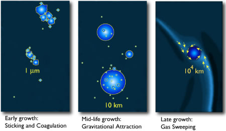
Our calculations use John Chambers’ Mercury integrator to follow the last evolutionary stages of a planetesimal swarm in the protoplanetary disk of a young low-mass red dwarf star. The underlying physical picture in the simulations is that the star and disk are of order one million years old. The initial stages of planet formation are assumed to already have been completed. Grains of solid material have stuck together to build larger and larger objects in the disk. Most of the gas that was originally in the disk has either accreted onto the star, or has been photoevaporated by high-energy photons from the star itself and the neighboring stars in the birth aggregate.

We’ve completed three sets of calculations, and our computers are currently working on a large number of additional runs. In the first set (containing sixty individual simulations) we assume that two Neptune-like giant planet cores have already managed to form beyond the protostellar ice line, where the temperature is lower than 150K, and where planets can grow more quickly because of the availability of ices. We also assume that the innermost Neptune-mass core has been able to migrate a small ways inward to a distance of ~0.2 AU from the central star. This situation was chosen so as to be in analogy with the known Neptune-mass planets orbiting the red dwarfs GL 436 and GL 581 (see yesterday’s post). In a second set of sixty simulations, we didn’t include the giant planet cores. In our simulations, the Neptune-mass cores assume a role similar to that which Jupiter and Saturn are believed to have had during the formation phases of the terrestrial planets in our own solar system.

In each of the 120 simulations that comprise the first two sets, we distribute 1000 planetesimals in initially circular orbits in the region between 0.04 AU and 0.12 AU surrounding the eventual stellar habitable zone for the 0.12 solar mass star. Each planetesimal contains 0.003 Earth masses (about a quarter of a lunar mass). The swarm of planetesimals is then allowed to evolve under its own self-gravity, the gravity of the star, and the gravity of the ice-giant cores (if they are present). Planetesimals that collide with each other are assumed to conserve total angular momentum in the collision, while merging into a larger composite body. Some planetesimals collide with the ice giants or with the star, or are thrown out of the system. In a typical simulation (shown below) the swarm rapidly works itself down over a period of a few thousand years into a system of several terrestrial mass planets. Earth-mass planets in the habitable zone of the star are a very common outcome of the simulations.

accretion simulation

In a third set (of thirty) simulations, we lowered the masses of the planetesimals to 0.0003 Earth-masses, that is, a factor of ten times lower. The results of these simulations were the formation of Mars-sized or smaller bodies in the stellar habitable zone.

The results have a simple interpretation. The final stages of terrestrial planet formation in the protoplanetary disks of red dwarf stars appears to be an efficient process. If one starts with an adequately high effective surface density of solid material in the disk, then one frequently gets Earth-mass planets in the habitable zone. If one starts with a lower surface density, then one gets final sets of terrestrial planets that (on average) have proportionally lower masses, i.e., no deal.

We believe that the key issue, then, is: what is the appropriate surface density to use?

If one makes reasonable extrapolations from the minimum-mass solar nebula that formed our own solar system, or if one extrapolates from the dust disks which are observed around young stars in the solar neighborhood (see the photo below of the disk orbiting AU Microscopium), then one should adopt a low surface density. This was the approach taken by Sean Raymond in his talk (which followed Ryan at AbSciCon). Sean’s results agreed quite well with our low-surface density simulations, namely, Mars-sized or smaller planets in the habitable zones of red dwarfs.

dust disk surrounding AU Microscopium

Submillimeter observations of dust masses in young stellar systems measure the amount of mass in dust, and are not directly sensitive to the amount of mass in large, planetesimal-sized bodies. Furthermore, such measurements give the dust mass at large distances (say greater than 1 astronomical unit at least) from the star, and hence do not give information about the mass of solids present in the innermost region of the disk.

Our preferred high surface density scenario is based on the “Minimum Mass Nebulae” for the inner regions of GJ 876 (0.32 solar mass), and Jupiter (0.001 solar mass). These are the two objects closest in mass to our hypothetical 0.12 solar mass star whose “terrestrial planet” systems we can measure.

In the case of Jupiter, the moon Io has a mass of 8.93e+25 grams, an orbital radius of 0.0028 AU, and an orbital period of 1.8 days. This implies a solid surface density of approximately 12,000 grams per square centimeter at the 1.8 day orbital radius in the proto-Jovian nebula.

In the case of GJ 876, planet “d” (which you can characterize from the actual Keck and Lick radial velocity data using the Systemic Console) has a mass of 4.5e+28 grams (7.5 Earth masses), an orbital radius of 0.02 AU, and an orbital period of 1.94 days. If we assume that GJ 876 d fed off material reaching out to a radius of 0.075 AU, then this implies a solid surface density of 11,000 grams per square centimeter at the 2.0 day orbital radius in GJ 876’s protoplanetary nebula. This is remarkably close to the value for Io. That is, the “rule of thumb” from these two systems suggests an effective surface density of solid material of ~10,000 grams per square centimeter at a 2-day orbital period.

The similarity between the solid surface densities obtained by grinding up Io and GJ 876d suggests that we also adopt a solid surface density of 11,000 grams per square centimeter at the 2-day orbital radius for our 0.12 solar mass star (0.015 AU). Using a reasonable r^-3/2 falloff in surface density as we move away from the star, this suggests a fiducial density of 2000 grams per square centimeter at a habitable-zone radius of 0.045 AU, which is the value that we use in our preferred (sets 1 and 2) simulations.

Once we’ve run a particular simulation, we choose a random angle from which the system is to be viewed. We then generate photometry that is typical of what high-end amateur observers such as Ron Bissinger or Tonny Vanmunster are capable of regularly achieving. For instance, here’s an example of Ron Bissinger’s observation of HD 149026b shortly after it was discovered.

We then “observe” the system by creating a simulated photometric time-series over a period of several hours, during the intervals in which a transit might possibly occur.

Our simulations imply about a 1.0% a-priori probability that a 0.12 solar mass red dwarf has a detectable, habitable planet. That means that most of the simulated systems, when observed at a random viewing angle, don’t show any transits:

simulated photometry of simulated system 18

With the omnipotence afforded by the simulation output files, we know that some of the simulations were not that far away from having a transiting planet:

simulated photometry of simulated system 1

Whereas some were closer still:

simulated photometry of simulated system 23

In this case, a tiny planet produces a grazing transit that is completely unobservable with 0.4% differential photometry:

simulated photometry of simulated system 47

And then, finally, gloriously:

simulated photometry of simulated system 42

That’s how I think we’ll get our first look at a truly habitable world orbiting an alien star.

Finally, back to the passage from John Herschel that starts this post off with an egregious bang. At first glance, it looks like a totally outrageous bit of self-serving grandstanding. Moreover, the quote itself is well-known to the extent that a reasonable person might justifiably press charges of second or even first degree cliche. On second glance, however, it actually seems rather appropriate.

Columbus thought he was headed for the East Indies, and he was justifying his expedition on an assumed distance from the Canary Islands to Japan of only 4444 km (as opposed to the true distance of 19,600 km). He had no conception whatever of America while he was still on the “far shores of Spain.”

Furthermore, the prediction of the existence of Neptune by Urbain Jean Joseph LeVerrier, was based on the large perturbations to the orbit of Uranus which occured from ~1810-1840, and which only occur once per Uranus-Neptune conjunction. The large derangement of Uranus’ orbit allowed LeVerrier to compute predicted ephemerides for the location of Neptune that were accurate enough for it to be quickly discovered by Johann Galle and Heinrich d’Arrest on the night of Sept. 23, 1846. LeVerrier was lucky, however. Even though he assumed an incorrect distance for Neptune of 36.15 AU, based on Bode’s spurious “law”, his method — which was essentially a laborious hand-cranked version of what goes on beneath the hood of the Systemic Console — was able to compensate for this incorrect assumption by invoking a mass for Neptune that was too large (2.9 times too large, in fact), and an eccentricity, e=0.11, that was also too large. Neptune’s actual orbit is currently nearly circular, with e=0.00884. As a result, LeVerrier’s orbital predictions of the location of Neptune in the skies of 1846 were close enough to allow it to be found, even though his predicted planet had an orbital period of 217 years, in comparison to Neptune’s actual period of only 166 years.

This point is often glossed over in the astronomical lore, and LeVerrier (with Adams invariably in tow) is lionized a bit too assiduously as a hero of the scientific method. In fact, luck, in the form of the fact that Uranus and Neptune happened to be close to conjunction, played a major, if not leading role. At the end of the day, we expect the same situation to hold true for those habitable planets transiting nearby low-mass red dwarf stars.

clouds

Habitable planets do have their drawbacks. For one, surface conditions near the triple point of water mean that the weather often interferes with differential photometry. That makes it hard for observers in the www.transitsearch.org collaboration to catch planet-bearing stars under clear dark skies during the time windows when transits are predicted to possibly occur!

cumulus clouds

Such was the case during the March 28, 2006 (06:59 UT) opportunity to check the low-mass red dwarf GL 581 for planetary transits. The planet orbiting GL 581 was announced by the Swiss Planet-hunting team last September (their discovery paper is here). GL 581b is one of the lowest-mass planets known outside our solar system. It’s likely similar in size and composition to Neptune or Uranus, with a minimum mass 17 times that of the Earth. The orbital period is 5.366 days, meaning that the surface temperature should be a bit under the boiling point of water. Tomorrow’s weather forecast for GL581b calls for cloudy skies, humidity near 100%, and afternoon highs near 180 F at the substellar point; the planet almost certainly spins once on its axis for every trip it makes around the star.

GL581 represents an ideal candidate for transitsearch.org observers, and there is no mention in the discovery paper that an attempt was made to check the star for planetary transits prior to the end of last year’s observing season. This lack of a transit check in the discovery paper makes sense, given the planet’s relatively low 3.6% a-priori transit probability, and the 5.366 day orbital period. Without a network of observers spread across the globe, it can take a very long time at a particular spot before one catches a transit window when the sky is (1) clear and (2) dark, and when the star is (3) high overhead. GL581b is a very exciting planet regardless of whether it transits, and so I’m sure Bonfils et al. just wanted to just get their discovery published in the literature. Papers “in prep.” garner no citations. Until Astronomy produces its first commercial killer apps, citations will remain the coin of the realm.

DSS2 Red Image of GL581

GL 581 is a springtime star, visible from both the Northern and Southern Hemispheres. There was an excellent opportunity last night for California observers to catch the transit, but the Golden State seems to have been clouded out from top to bottom. I have not gotten any reports of observations being made. The next windows of opportunity, and the best viewing sites are:

(1) April 2, 2006 19:04 UT — Japan, Australia
(2) April 8, 2006 00:33 UT — Europe, South Africa
(3) April 13, 2006 09:20 UT — North, South America

The transitsearch.org network has participants in all of these locations, so we should be set.

Boy oh boy would it be a big deal if GL 581b turns out to transit. The occurence of transits would fix the inclination of the planetary orbit, which would eliminate the sin(i) degeneracy that currently plagues the mass estimate. If the planet transits, we would know that it truly has a Neptune mass. The depth of the transit would give us the planetary size, which, coupled with the mass, would yield the density. The density would tell us what the planet is made of. If it is primarily water, like Uranus or Neptune, then we expect a radius of ~0.3 Jupiter radii. If the planet is made of rock and metal, however, like the terrestrial planets in our solar system, then the radius will be smaller, more in the neighborhood of ~0.22 Jupiter radii. A water-rich composition would tell us that the planet formed further away from the star, and then migrated inward to its steamy current location. This information, in turn, would give us valuable insight into the conditions that held sway in the disks surrounding low mass stars, and would help guide our hypotheses regarding the presence of habitable worlds orbiting the lowest mass stars.

Hopefully we’ll snag a transit on April 2nd and then confirm it on April 8th and April 13th. If that happens, I’ll mail a dollar to every registered user of oklo.org. With roulette wheel-like 3.6% odds, I’m not exactly betting the house, but nonetheless, hope springs eternal!

If you are interested in participating in transitsearch.org, feel free to subscribe to the (moderated) transitsearch.org observers list.