hd 20782 oct 20, 2006 (3.6%)

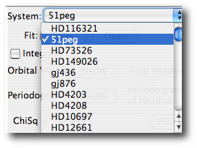
As advertised in yesterday’s post, three newly published radial velocity data sets have just been added to the system menu of the Systemic Console, and to the www.transitsearch.org candidates list. The data set for HD20782, published by Jones et al. of the Anglo-Australian Planet Search, is definitely the most interesting of the trio. Let’s work the HD 20782 velocities over with the console, and see what they have to say.

sunset

First, fire up the console. (If you use Firefox on Windows, and you’ve had success getting the console to work with that particular line-up, please post a response in answer to Vincent’s comment on yesterday’s post. All of Aaron’s oklo.org Java development has been done on Mac OSX using Safari. Also, we’ve had many reports that the console works well with Internet Explorer on Windows, so if Firefox won’t run the Java, give IE a try. And could someone ask Mr. Bill G. to send me a check for that plug?)

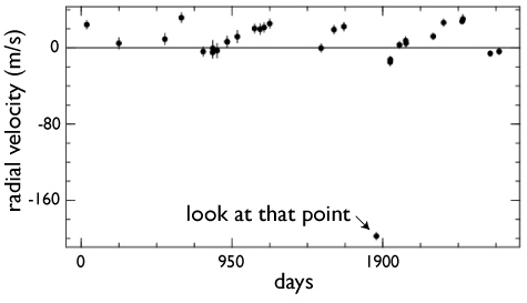
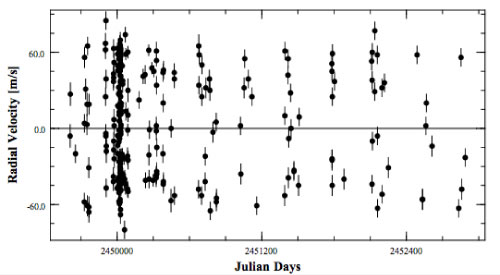
At any rate, the HD 20782 radial velocity data set has one data point that sticks down like a sore thumb:

velocities

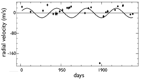
Activation of one planet and a little bit of fooling around with circular orbits shows that even when the discrepant point is ignored, the waveform of the planet is not at all sinusoidal. The points contain an almost sawtooth-like progression:

circular orbit fit

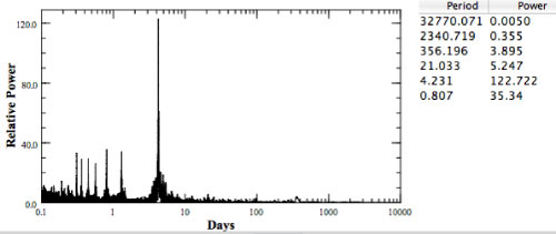
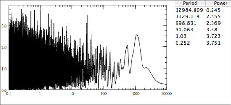
Because of the non-sinusoidal nature of the velocities, the periodogram (obtained by clicking the periodogram button) is rather uninformative. There’s a lot of power in a lot of different peaks, and it’s not immediately clear what is going on planet-wise:

periodogram

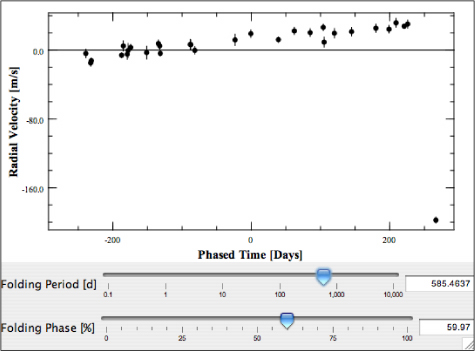
Aaron has been working very hard on console development, and we will soon release an updated version with a number of absolutely bling features. Ever wondered what your fits sound like? One new feature is a “folding window”, which allows the data to be phased at whatever period one likes. The folding window is very useful for data-sets of the type produced by HD 20782. It quickly reveals that something like a 600 day periodicity brings out the overall shape of the planetary waveform:

folding window

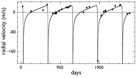
Using 600 days as the basis for a 1-planet fit, activating eccentricity, and using a combination of slider work, 1-d minimization, and Levenberg-Marquardt, eventually produces excellent fits to the data that look like this:

fit to hd20872

Jones et al., for example, in their discovery paper, report an orbital period of P=585.86 days, an eccentricity, e=0.92, a mass (times the sine of the unknown orbital inclination) of Msin(i)=1.8 Jupiter masses, and a longitude of periastron of 147 degrees.

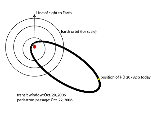
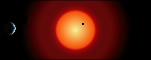
This planet is one bizzare world, and seems to be very similar to HD 80606 b (another oklo.org favorite). The orbital period is 1.6 years. The planet spends most of it’s time out at ~2.6 AU. In our solar system, this distance is out beyond Mars in the inner asteroid belt. Once per orbit, however, HD 20782 b comes swinging in for a steamy encounter with the star. The periastron distance is a scant 0.11 AU, roughly half Mercury’s distance from the Sun. The planet is likely swathed in turbulent white water clouds. Raindrops vaporize as the star looms larger and larger in the sky.

Stars that loom large in alien skies are good news for transitsearch.org, and in the case of HD 20782 b, we here on earth are particularly fortunate. HD 20782 b’s line of apsides lies within about 60 degrees of alignment with the line of sight to the Earth. This raises the a-priori geometric probability of having a transit observable from Earth to a relatively high 3.6%. (The a-priori probability of transit for a planet with a 1.6-year period and a circular orbit is only ~0.3%).

oribital figure

high e

The ante keeps going up. 5 Ghz on the desktop. A resolution to write a new oklo post every day. An alarmingly effective new .php-based approach over at Jean Schneider’s Extrasolar Planets Encyclopaedia. The rapidly increasing rate of planet detection is causing the census of extrasolar planets to close in fast on the two hundred mark. Weird new worlds uncovered by the microlensing collaboration and the OGLE wide-field transit survey are starting to accumulate in the electronic annals of astro-ph. The radial velocity programs are cranking up their productivity with high-yield surveys like N2K. And we here at oklo.org have to stay on our toes to keep the transitsearch.org candidates table and the Systemic Console system list up to date.

Live fitting with the Systemic Console

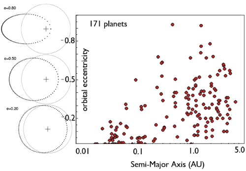
The rapidly growing collection of extrasolar planets is really starting to crowd the semi-major axis — eccentricity, or “a-e“, diagram. This (very nearly) up-to-date version shows 171 planets detected with the radial velocity technique, with e=0.2, e=0.5, and e=0.8 orbital figures shown on the y-axis for reference:

latest tally of extrasolar planets

The swarm of planets in the above a-e diagram includes three newly announced (and very interesting) new systems whose radial velocity data sets have just been added to the console’s system menu: HD 187085, HD 20782, and HD 45350. I’ll check back soon with a detailed discussion of these planets and their implications, but in the meantime, try using the Systemic Console to fit them.

One last thing: I was at a meeting last week where there was a Windows-based machine sitting on the table in front of me. When I brought up the www.oklo.org in Internet Explorer, I was aghast to see that the menu of links (which you should see to your right) had been pushed all the way down to the bottom of the page. I had to scroll all the way down to even see it. We thought we had fixed this problem, but apparently not. We’re working on it. Also, if you are a Macintosh user, run the console in Safari. There is a still a Java issue with the Firefox on OS X. Firefox should, however, work fine on both Linux and Windows machines if your Java libraries are up to date…

A Case for Habitable Planets Orbiting Red Dwarfs

“The past year has given to us the new [minor] planet Astraea; it has done more – it has given us the probable prospect of another. We see it as Columbus saw America from the far shores of Spain. Its movements have been felt, trembling along the far-reaching line of our analysis with a certainty hardly inferior to ocular demonstration.”

— Sir John Herschel addressing the British Association of the Advancement of Science on Sept. 15, 1846, two weeks prior to the discovery of Neptune.

Yesterday, Ryan Montgomery gave his presentation at the AbSciCon meeting in Washington DC, and laid forth our provocative hypothesis. We think that Earth-mass planets are common in the habitable zones of the lowest-mass red dwarf stars, and we think that these planets can potentially be detected by targeted photometric searches of the nearest known low-mass stars. The closest stars on this list are accessible to transitsearch.org observers, and we are advocating that the search begin immediately.
Earth from Space

Our calculations use John Chambers’ Mercury integrator to follow the last evolutionary stages of a planetesimal swarm in the protoplanetary disk of a young low-mass red dwarf star. The underlying physical picture in the simulations is that the star and disk are of order one million years old. The initial stages of planet formation are assumed to already have been completed. Grains of solid material have stuck together to build larger and larger objects in the disk. Most of the gas that was originally in the disk has either accreted onto the star, or has been photoevaporated by high-energy photons from the star itself and the neighboring stars in the birth aggregate.

We’ve completed three sets of calculations, and our computers are currently working on a large number of additional runs. In the first set (containing sixty individual simulations) we assume that two Neptune-like giant planet cores have already managed to form beyond the protostellar ice line, where the temperature is lower than 150K, and where planets can grow more quickly because of the availability of ices. We also assume that the innermost Neptune-mass core has been able to migrate a small ways inward to a distance of ~0.2 AU from the central star. This situation was chosen so as to be in analogy with the known Neptune-mass planets orbiting the red dwarfs GL 436 and GL 581 (see yesterday’s post). In a second set of sixty simulations, we didn’t include the giant planet cores. In our simulations, the Neptune-mass cores assume a role similar to that which Jupiter and Saturn are believed to have had during the formation phases of the terrestrial planets in our own solar system.

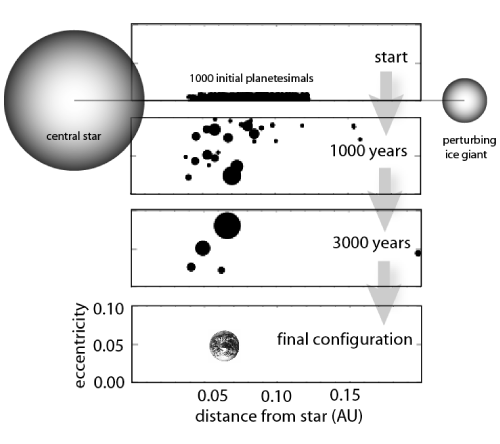
In each of the 120 simulations that comprise the first two sets, we distribute 1000 planetesimals in initially circular orbits in the region between 0.04 AU and 0.12 AU surrounding the eventual stellar habitable zone for the 0.12 solar mass star. Each planetesimal contains 0.003 Earth masses (about a quarter of a lunar mass). The swarm of planetesimals is then allowed to evolve under its own self-gravity, the gravity of the star, and the gravity of the ice-giant cores (if they are present). Planetesimals that collide with each other are assumed to conserve total angular momentum in the collision, while merging into a larger composite body. Some planetesimals collide with the ice giants or with the star, or are thrown out of the system. In a typical simulation (shown below) the swarm rapidly works itself down over a period of a few thousand years into a system of several terrestrial mass planets. Earth-mass planets in the habitable zone of the star are a very common outcome of the simulations.
accretion simulation

In a third set (of thirty) simulations, we lowered the masses of the planetesimals to 0.0003 Earth-masses, that is, a factor of ten times lower. The results of these simulations were the formation of Mars-sized or smaller bodies in the stellar habitable zone.

The results have a simple interpretation. The final stages of terrestrial planet formation in the protoplanetary disks of red dwarf stars appears to be an efficient process. If one starts with an adequately high effective surface density of solid material in the disk, then one frequently gets Earth-mass planets in the habitable zone. If one starts with a lower surface density, then one gets final sets of terrestrial planets that (on average) have proportionally lower masses, i.e., no deal.

We believe that the key issue, then, is: what is the appropriate surface density to use?

If one makes reasonable extrapolations from the minimum-mass solar nebula that formed our own solar system, or if one extrapolates from the dust disks which are observed around young stars in the solar neighborhood (see the photo below of the disk orbiting AU Microscopium), then one should adopt a low surface density. This was the approach taken by Sean Raymond in his talk (which followed Ryan at AbSciCon). Sean’s results agreed quite well with our low-surface density simulations, namely, Mars-sized or smaller planets in the habitable zones of red dwarfs.
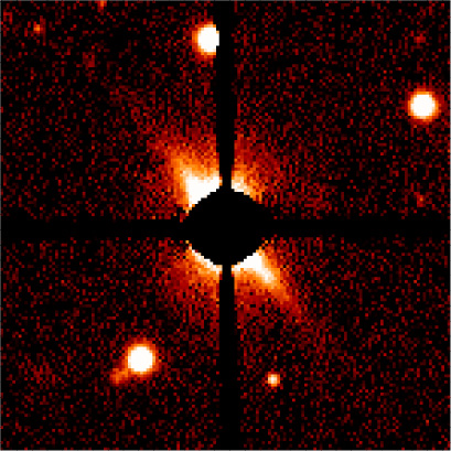
dust disk surrounding AU Microscopium

Submillimeter observations of dust masses in young stellar systems measure the amount of mass in dust, and are not directly sensitive to the amount of mass in large, planetesimal-sized bodies. Furthermore, such measurements give the dust mass at large distances (say greater than 1 astronomical unit at least) from the star, and hence do not give information about the mass of solids present in the innermost region of the disk.

Our preferred high surface density scenario is based on the “Minimum Mass Nebulae” for the inner regions of GJ 876 (0.32 solar mass), and Jupiter (0.001 solar mass). These are the two objects closest in mass to our hypothetical 0.12 solar mass star whose “terrestrial planet” systems we can measure.

In the case of Jupiter, the moon Io has a mass of 8.93e+25 grams, an orbital radius of 0.0028 AU, and an orbital period of 1.8 days. This implies a solid surface density of approximately 12,000 grams per square centimeter at the 1.8 day orbital radius in the proto-Jovian nebula.

In the case of GJ 876, planet “d” (which you can characterize from the actual Keck and Lick radial velocity data using the Systemic Console) has a mass of 4.5e+28 grams (7.5 Earth masses), an orbital radius of 0.02 AU, and an orbital period of 1.94 days. If we assume that GJ 876 d fed off material reaching out to a radius of 0.075 AU, then this implies a solid surface density of 11,000 grams per square centimeter at the 2.0 day orbital radius in GJ 876’s protoplanetary nebula. This is remarkably close to the value for Io. That is, the “rule of thumb” from these two systems suggests an effective surface density of solid material of ~10,000 grams per square centimeter at a 2-day orbital period.

The similarity between the solid surface densities obtained by grinding up Io and GJ 876d suggests that we also adopt a solid surface density of 11,000 grams per square centimeter at the 2-day orbital radius for our 0.12 solar mass star (0.015 AU). Using a reasonable r^-3/2 falloff in surface density as we move away from the star, this suggests a fiducial density of 2000 grams per square centimeter at a habitable-zone radius of 0.045 AU, which is the value that we use in our preferred (sets 1 and 2) simulations.

Once we’ve run a particular simulation, we choose a random angle from which the system is to be viewed. We then generate photometry that is typical of what high-end amateur observers such as Ron Bissinger or Tonny Vanmunster are capable of regularly achieving. For instance, here’s an example of Ron Bissinger’s observation of HD 149026b shortly after it was discovered.

We then “observe” the system by creating a simulated photometric time-series over a period of several hours, during the intervals in which a transit might possibly occur.

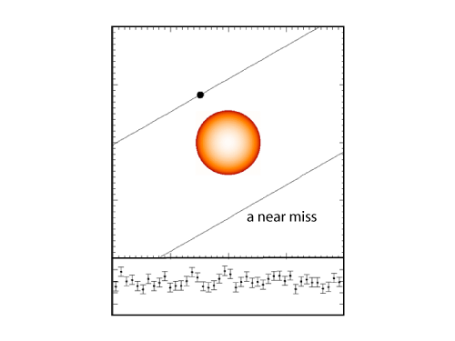
Our simulations imply about a 1.0% a-priori probability that a 0.12 solar mass red dwarf has a detectable, habitable planet. That means that most of the simulated systems, when observed at a random viewing angle, don’t show any transits:
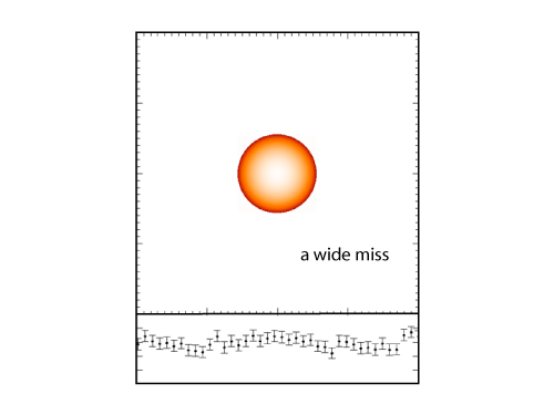
simulated photometry of simulated system 18

With the omnipotence afforded by the simulation output files, we know that some of the simulations were not that far away from having a transiting planet:
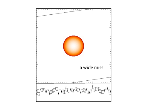
simulated photometry of simulated system 1

Whereas some were closer still:

simulated photometry of simulated system 23

In this case, a tiny planet produces a grazing transit that is completely unobservable with 0.4% differential photometry:
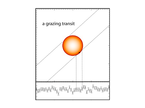
simulated photometry of simulated system 47

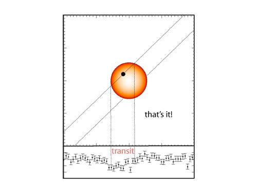
And then, finally, gloriously:

simulated photometry of simulated system 42

That’s how I think we’ll get our first look at a truly habitable world orbiting an alien star.

Finally, back to the passage from John Herschel that starts this post off with an egregious bang. At first glance, it looks like a totally outrageous bit of self-serving grandstanding. Moreover, the quote itself is well-known to the extent that a reasonable person might justifiably press charges of second or even first degree cliche. On second glance, however, it actually seems rather appropriate.

Columbus thought he was headed for the East Indies, and he was justifying his expedition on an assumed distance from the Canary Islands to Japan of only 4444 km (as opposed to the true distance of 19,600 km). He had no conception whatever of America while he was still on the “far shores of Spain.”

Furthermore, the prediction of the existence of Neptune by Urbain Jean Joseph LeVerrier, was based on the large perturbations to the orbit of Uranus which occured from ~1810-1840, and which only occur once per Uranus-Neptune conjunction. The large derangement of Uranus’ orbit allowed LeVerrier to compute predicted ephemerides for the location of Neptune that were accurate enough for it to be quickly discovered by Johann Galle and Heinrich d’Arrest on the night of Sept. 23, 1846. LeVerrier was lucky, however. Even though he assumed an incorrect distance for Neptune of 36.15 AU, based on Bode’s spurious “law”, his method — which was essentially a laborious hand-cranked version of what goes on beneath the hood of the Systemic Console — was able to compensate for this incorrect assumption by invoking a mass for Neptune that was too large (2.9 times too large, in fact), and an eccentricity, e=0.11, that was also too large. Neptune’s actual orbit is currently nearly circular, with e=0.00884. As a result, LeVerrier’s orbital predictions of the location of Neptune in the skies of 1846 were close enough to allow it to be found, even though his predicted planet had an orbital period of 217 years, in comparison to Neptune’s actual period of only 166 years.

This point is often glossed over in the astronomical lore, and LeVerrier (with Adams invariably in tow) is lionized a bit too assiduously as a hero of the scientific method. In fact, luck, in the form of the fact that Uranus and Neptune happened to be close to conjunction, played a major, if not leading role. At the end of the day, we expect the same situation to hold true for those habitable planets transiting nearby low-mass red dwarf stars.
clouds

Habitable planets do have their drawbacks. For one, surface conditions near the triple point of water mean that the weather often interferes with differential photometry. That makes it hard for observers in the www.transitsearch.org collaboration to catch planet-bearing stars under clear dark skies during the time windows when transits are predicted to possibly occur!

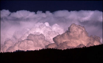
cumulus clouds

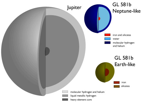
Such was the case during the March 28, 2006 (06:59 UT) opportunity to check the low-mass red dwarf GL 581 for planetary transits. The planet orbiting GL 581 was announced by the Swiss Planet-hunting team last September (their discovery paper is here). GL 581b is one of the lowest-mass planets known outside our solar system. It’s likely similar in size and composition to Neptune or Uranus, with a minimum mass 17 times that of the Earth. The orbital period is 5.366 days, meaning that the surface temperature should be a bit under the boiling point of water. Tomorrow’s weather forecast for GL581b calls for cloudy skies, humidity near 100%, and afternoon highs near 180 F at the substellar point; the planet almost certainly spins once on its axis for every trip it makes around the star.

GL581 represents an ideal candidate for transitsearch.org observers, and there is no mention in the discovery paper that an attempt was made to check the star for planetary transits prior to the end of last year’s observing season. This lack of a transit check in the discovery paper makes sense, given the planet’s relatively low 3.6% a-priori transit probability, and the 5.366 day orbital period. Without a network of observers spread across the globe, it can take a very long time at a particular spot before one catches a transit window when the sky is (1) clear and (2) dark, and when the star is (3) high overhead. GL581b is a very exciting planet regardless of whether it transits, and so I’m sure Bonfils et al. just wanted to just get their discovery published in the literature. Papers “in prep.” garner no citations. Until Astronomy produces its first commercial killer apps, citations will remain the coin of the realm.

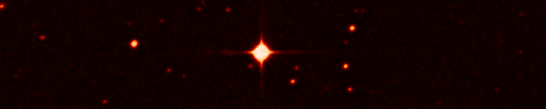
DSS2 Red Image of GL581

GL 581 is a springtime star, visible from both the Northern and Southern Hemispheres. There was an excellent opportunity last night for California observers to catch the transit, but the Golden State seems to have been clouded out from top to bottom. I have not gotten any reports of observations being made. The next windows of opportunity, and the best viewing sites are:

(1) April 2, 2006 19:04 UT — Japan, Australia
(2) April 8, 2006 00:33 UT — Europe, South Africa
(3) April 13, 2006 09:20 UT — North, South America

The transitsearch.org network has participants in all of these locations, so we should be set.

Boy oh boy would it be a big deal if GL 581b turns out to transit. The occurence of transits would fix the inclination of the planetary orbit, which would eliminate the sin(i) degeneracy that currently plagues the mass estimate. If the planet transits, we would know that it truly has a Neptune mass. The depth of the transit would give us the planetary size, which, coupled with the mass, would yield the density. The density would tell us what the planet is made of. If it is primarily water, like Uranus or Neptune, then we expect a radius of ~0.3 Jupiter radii. If the planet is made of rock and metal, however, like the terrestrial planets in our solar system, then the radius will be smaller, more in the neighborhood of ~0.22 Jupiter radii. A water-rich composition would tell us that the planet formed further away from the star, and then migrated inward to its steamy current location. This information, in turn, would give us valuable insight into the conditions that held sway in the disks surrounding low mass stars, and would help guide our hypotheses regarding the presence of habitable worlds orbiting the lowest mass stars.

Hopefully we’ll snag a transit on April 2nd and then confirm it on April 8th and April 13th. If that happens, I’ll mail a dollar to every registered user of oklo.org. With roulette wheel-like 3.6% odds, I’m not exactly betting the house, but nonetheless, hope springs eternal!

If you are interested in participating in transitsearch.org, feel free to subscribe to the (moderated) transitsearch.org observers list.

HD 149026

The Solar System was once a gigantic black cloud in space, imbued with a tiny overall spin in some particular random direction. The net spin of our ancient protostellar cloud is still manifest in today’s solar system. The planets all orbit the Sun in a direction counterclockwise as seen from above. The major planetary satellites (with the exception of Triton) all orbit counterclockwise as well. The Sun spins on an axis that lies within 7 degrees of the average orbital plane of the planet.

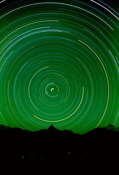
Star trails

The law of conservation of momentum suggests that alien planetary systems should display a similar state of orbital affairs. When a planetary system forms more or less quiescently, and more or less in isolation, then the final spin axis of the parent star should be nearly perpendicular to the orbital plane of the planets.

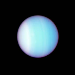
If the stellar equator and the planetary orbital planes are far from alignment, then we have evidence that disruptive events occurred early in the history of the planetary system. Spin-orbit misalignment hints at planetary collisions, ejections, and other dramatic events. In the Solar System, for example, the crazy 97.77 degree tilt of Uranus’ polar axis may be evidence that a large (perhaps Earth-mass) object collided with Uranus early in its history, leaving its spin axis askew, and its poles bathed in an endless succession 42-year days.

HST photo of Uranus

In a new paper accepted for publication in the Astrophysical Journal, members of the systemic team have participated in an investigation of the spin-orbit alignment of the recently discovered transiting planet orbiting HD149026. Our goal was to get a better sense of whether this star-planet system suffered a catastrophe in its distant past.

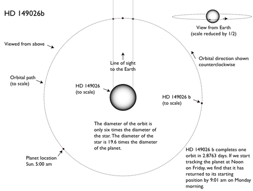
HD 149026 b was discovered last year by N2K (the discovery paper is here). The planet has a mass ~114 times that of the Earth (slightly bigger than Saturn) and has a 2.875 day orbital period. By measuring how the star’s light dims as the planet passes in front of the star, it’s possible to determine the size and the exact orbital geometry for the system. Here’s a scale model in which the star, and the planet, and the orbit are all shown in their correct proportions:

The HD 149026 planetary system

Perhaps the most charming aspect of HD 149026 b (to the limited extent that a scalding 1600K planet can exert charm) is that the planetary sidereal year lasts exactly one weekend. That is, if you punch a clock at noon on Friday, the planet has made one full orbit at 9:01 am the following Monday.

Perhaps the most scientifically interesting aspect of HD 149026 b is its small size. The transit depth is only 0.3%, which implies that the planet has a radius of only ~0.7 Jupiter radii. That is surprisingly small, given the high temperature on the planetary surface, and tells us that the planet is quite dense. It needs to contain at least 50 Earth masses of elements heavier than hydrogen and helium. This huge burden of heavy elements is hard to explain. One possibility is that the planet was built up from the collision of several Uranus or Neptune like objects. If this were the case, then one might expect that the final orbital plane could be significantly misaligned with the equatorial plane of the star.

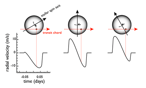
Our measurement of the spin-orbit alignment for HD 149026 makes use of a phenomenon known as the Rossiter-McLaughlin effect. In 1924, Rossiter and McLaughlin independently measured the spin-orbit alignment of the eclipsing binary systems beta-Lyrae and Algol by modeling the variations in the measured radial velocities of the stars during transit. This effect, now appropriately called the Rossiter-McLaughlin effect, occurs any time an object (star or planet) occults part of a rotating stellar surface. The following figure shows how a rotating star outputs a small red-blue shifted version of its spectrum as we examine the changing radial spin-velocity from one limb to the other. When a planet passes in front of the oncoming limb, it blocks out red-shifted light, while the planet blocks out blue-shifted light when covering the outgoing limb. This is interpreted by the radial velocity code as a positive and then negative shift in the radial velocity of the star. The amplitude of this effect is thus due both to the spin velocity of the star as well as the total flux blocked out during transit.

schematic diagram showing rossiter effect

The Rossiter effect can be used to tell us how closely the stellar equator is aligned to with the orbital plane of the planet. When the planet’s path across the stellar disk is not parallel to the stellar equator, the radial velocity zero-point does not occur at the transit mid-point, and the radial velocity curve is asymmetric. The figure above illustrates how this works.

High-cadence radial velocity observations taken during a transit are required to accurately measure the Rossiter effect. The in-transit velocities can be combined with other data, including the out-of-transit radial velocities which constrain the planetary orbit, and the transit photometry. An overall coupled model of all of these data can then give us the best possible picture of the system. Our new paper describes the exact details of how such an overall model can be constructed for HD 149026. The end result is that the equator of the star and the orbital plane of the transiting planet are quite well aligned; we measure the value of the misalignment angle to be 11 plus or minus 14 degrees.

Although a fourteen degree (1-sigma) uncertainty is more than we’d like, it nevertheless provides an excellent constraint on the HD 149026 system. Since the misalignment of our own sun is ~7 degrees relative to the net planetary orbital angular momentum, and because we believe that the solar system formed fairly quiescently, we are primarily interested in whether HD 149026 b sports a severe misalignment (say 40 degrees or more). From our modelling, it’s clear that the orbit and planetary spin are not egregiously out of whack. Hence, there’s no evidence of a particularly disruptive formation history. That is, no catastrophic orbit altering collisions between massive protostellar cores. Rather, we are left with evidence of a more traditional, more mundane history, in which planetary formation was dominated by gradual accretion and the prolonged interactions with a planetary disk

And the mystery of HD 149026b’s large core persists. How did all those heavy elements — all that oxygen, nitrogen, carbon, iron, gold, get into the planet?

Our favored explanation draws on a scenario described by Frank Shu in 1995, in which the planetesimal migrates radially inward through the planetary disk until it reaches the interior 2:1 resonance with the “magnetic X-point,” the outermost point at which closed stellar magnetic field lines intersected the planetary disk. At the X-point, heated ionized gas is forced to leave the disk and climb up the field lines to accrete directly onto the star. In this occurs, the planetismal is stuck in a gas-starved environment for the remainder of the disk lifetime, and is essentially fed nothing but rocks and heavy elements for millions of years. The end result is a crazy-large 72 Earth-mass core in the middle of a 114 Earth-mass planet.

stop-action stop-gap

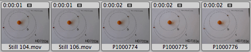
stills from the 73526 animation

We’ve noticed that fresh content encourages regular return visits to oklo.org.

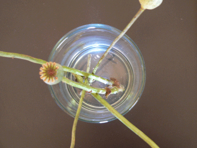
With that sentiment in mind, here’s a stop-action .mpeg4 animation of the newly discovered 2:1 resonant planetary system orbiting HD73526. The planets are represented by red and green peppercorns, and a kumquat stands in for the central star:

hd73526.mov

If the version above won’t load in your browser, try this one. Rest assured that the systemic team is hard at work on more substantive posts (including some very interesting new exoplanet-related results), so check back frequently!

analog

It’s been unseasonably cold in Santa Cruz. Last night, a freak hailstorm left drifts of icy planetesimals lodged between the leaves of the banana tree outside the bedroom window.

My office, however, is nice and warm. This is because two 2.5 Ghz G5 processors are running mercury.f at full tilt to simulate the formation of habitable planets orbiting low-mass red dwarf stars. The calculations are being done in preparation for Ryan Montgomery’s presentation at AbSciCon in Washington D.C. Two weeks to go.
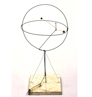
Calder, 1931, Two Spheres Within A Sphere

Two Spheres Within A Sphere Alexander Calder, 1931

Most of the runs have already been carried out using a linux-based beowulf cluster, which is able to run more than 100 individual simulations at once. Each of these simulations starts with 1000 low-mass planetesimals, and calculates the final stages of terrestrial planet formation by allowing the orbiting planetesimals to interact under their mutual gravitational influence. Collisions and ejections gradually winnow the initial swarm down to a few surviving terrestrial mass planets. By doing many simulations, we build up a statistical picture of what the distribution of red dwarf planetary systems should look like.

The desktop computer contains the fastest individual processors to which we have full access. We’ve therefore harnessed it for a single test-case run to investigate the overall sensitivity of our results to the number of initial particles. The processors have spent the last six weeks evolving a system that had an initial distribution of 10,000 small planetesimals. At the projected rate of evolution, it should just manage to finish up just in time. Indeed, if you see Ryan hunched over his laptop at the conference, you’ll know what he’s up to.

John Chambers’ Mercury code (like the Systemic Console in integrator mode) is based on the method of direct summation. At each timestep, each particle in the simulation experiences a gravitational attraction of the form GM/r^2 from every other body in the system. For a 10,000 particle system, that means of order ((10,000)x(9,999))/2=49,995,000 square roots must be computed every timestep (and the actual number is higher, because each timestep consists of a considerable number of substeps). As the number of particles increases, the cost of the calculation increases as the number of particles squared. Our 10,000 particle simulation is 100 times more expensive than the 1,000 particle production runs, and thus pushes the limits of what we can currently readily do.

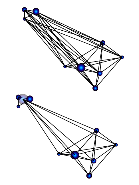
Many problems in gravitational N-body dynamics can be solved without resorting to direct summation. In essence, this is because to a high degree of approximation, the gravitational attraction from distant particles depends only on the the rough location and total mass of the distant particles. One gets nearly the same result by lumping distant particles into a single, equivalent, large-mass particle:

nbody connections

Using clever variations of this basic idea, one can speed up an N-body (or equivalently, an SPH) calculation enormously. Competitive N-body codes for large-N problems, such as the collisions of galaxies or the formation of structure in the early universe, generally scale as N log(N). For large N, the difference between N^2 and N log(N) is profound. With a million particles, for example, an N log(N) calculation is a cool 72,382 times faster than the brute-force N^2 approach.

One might ask, is there a way to further speed up the computation of the gravitational forces so that finding the accelerations becomes an order N process?

Remarkably, an order-N computational N-body method was employed by Erik Holmberg of the Lund Observatory in Sweden in 1941. Instead of integrating the equations of motion with a computer, Holmberg modeled a two-dimensional system of gravitating particles as an actual physical distribution of movable light bulbs laid out on a gridded sheet of dark paper! Because the intensity of light from a point source diminishes as 1/r^2, one can directly relate the intensity of the light at a particular spot to the gravitational acceleration. The order-N^2 process of computing the gravitational force on a given particle from all of the other particles reduces to a measurement of the total intensity of light in two perpendicular directions using a photocell and a galvanometer. Since one set of measurements is required for the location of each light bulb, the method scales as N. Here is a link to Holmberg’s paper. It’s one of my all-time favorites.

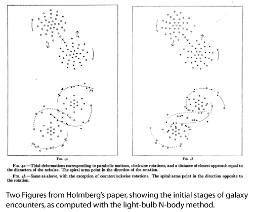
With his analog method for computing the net gravitational acceleration on each of his light bulb “point masses”, Holmberg could compute the change in trajectories which would occur over a time interval using a simple integration scheme such as Euler’s method. A timestep would then be completed by moving all of the light bulbs to their updated positions, at which point a new estimate of the gravitational acceleration could be made. Holmberg’s scheme allowed him to gain a better understanding of important aspects of the dynamics of close encounters between disk galaxies, including the phenomena of orbital decay and the formation of tidal tails:

results of Holmberg's integrations.

There is an interesting lesson to be drawn. Use of an analog method reduces an N^2 direct summation computation to order N, foreshadowing a time when quantum computation will similarly reduce the computational time for direct summation from N^2 to N. Until that time, however, the light-bulb method beats all others as the number of particles approaches an arbitrarily large value.

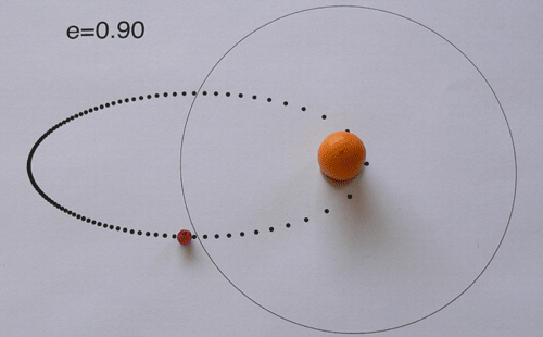
In honor of analog methods, here’s a home-made mpeg-4 stop-action animation of a peppercorn orbiting a kumquat in an ellipse with e=0.90. (Try this version if the other one loads a screen of gibberish).

peppercorn orbiting a kumquat.

octave

A very interesting new planetary system has been discovered in orbit around the nearby star HD 73526, a solar-type main sequence dwarf visible from the Southern Hemisphere. The discovery was made by Chris Tinney, Paul Butler, Geoff Marcy and their collaborators on the Anglo Australian Planet Search Project. The discovery paper has been accepted by the Astrophysical Journal, and a preprint describing the discovery has been posted to arXiv.org.

photo credit: Adriane Steinacker

[Photo of persimmons at Rakushisha, Kyoto, Japan, c2005 Adriane Steinacker]

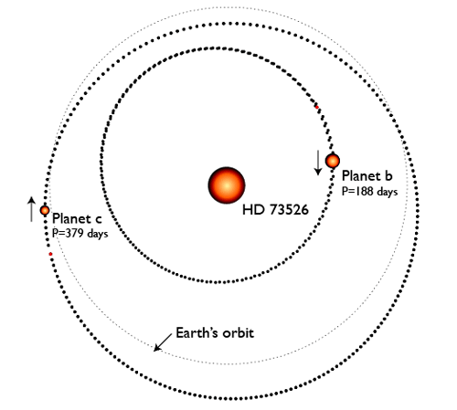
The system contains two giant planets. The inner, slightly more massive planet (imaginatively named “b”) contains at least 3 Jupiter masses, and orbits with a 188 day period. The outer planet, c, is only slightly less massive, with about 2.5 Jupiter masses. It orbits with a period of roughly 379 days. Planet c is a true room temperature gas giant. Liquid water likely blows in gusty sheets across its cloudy skies. (And it’s worth noting that any large moons circling HD 73526 c lie pleasantly within the stellar habitable zone.)

orbits of HD 73526 b and c

The large masses of the two planets, and their relatively small orbital separation, indicate that they exert strong perturbations on each other’s motion. It appears that in order for the system to be stable, it is required that b and c exist in a protective 2:1 resonance. In other words, on average, planet c circles the parent star exactly half as many times as does planet b. Amazingly, however, it appears that the periastron points of the two orbits are not locked in sync, but rather circulate at very different rates around the star. This situation leads to a bizarre orbital motion when plotted over thousands of years. I’ve made an mpeg animation which shows how this works. In the animation, the clockhand like lines show the periastron angles of the orbits. They undergo a crazy, almost drunken, dance, but somehow, the system configuration manages to remain stable indefinitely.

I’ve also added the published radial velocity data for HD 73526 to the Systemic Console. Take a peek at the published orbital parameters (both Keplerian and dynamical) if you have a hard time rolling the Console’s Levenberg-Marquardt algorithm into the best-fit configuration. I will put up a post shortly which goes into more detail about the dynamics of this fascinating system and what they tell us about planetary formation.

M

This post follows up post #14, The Next Big Thing.

proxima centauri

In 1916, in circular #30 of South Africa’s Union Observatory , Robert T. A. Innes reported the discovery of a faint red star in Centaurus. This otherwise unremarkable star, more than 100 times too faint to be seen with the naked eye, attracted his attention because it was rapidly moving with respect to other stars in the same part of the sky. This large proper motion indicated that the star was almost certainly a close neighbor of the Sun, and in 1917, this suggestion was verified. The distance to the star was measured to be only 4.22 light years, closer to the Sun than any other known star. Its extremely faint appearance, in spite of its close proximity, made it the intrinsically least luminous star known to astronomy at that time.

Proxima Centauri, as the star was later named, is now known to be merely the nearest (and most famous) of the roughly 50 billion red dwarfs (also called M-dwarfs) which inhabit our galaxy.

What about planets? Is it possible to have a terrestrial planet in orbit around Proxima? Do red dwarfs have a shot at harboring life-bearing worlds? If such worlds exist can we detect them?

Yes.

(more…)

disks

The black cloud post describes how the formation of a star and a planetary system can be traced back to the moment when a dense core within a giant molecular cloud begins to suffer an inside-out collapse. The gas at the center of the cloud collapses first, and congregates into the beginnings of a hydrostatically supported protostar. The overlying regions thus lose their support and begin to career inward as well. A wave of collapse radiates outward from the center of the cloud, triggering a downward avalanche of gas and dust. Computer simulations show how gas that has fallen from large distances comes together to form a protostellar disk in orbit around the nascent central protostar. In the image shown below, a simulation of the earliest phases of our own solar system show a region (viewed edge-on) that is several hundred astronomical units across, and plotted 40,000 years after the collapse has started. At this stage of the simulation, roughly half of a solar mass of material has collected in the central protostar, and another half a solar mass or so is orbiting in a very massive protostellar disk.

Computer simulation showing gas infall onto a protostellar disk.

As the disk grows in mass, it begins to feel its own self-gravity, and some regions begin to collapse under their own weight. At the same time, the pressure of the gas in the disk resists the tendancy to collapse, and the differential rotation of the disk acts to sheer out fragments as they grow. This process can also be simulated, and the result is spiral waves (viewed here from above):

Simulation showing the development of spiral waves in a self-gravitating disk

The presence of the spiral waves causes angular momentum to be transferred outward through the disk, while allowing the majority of the mass to flow inward to eventually join with the central protostar. Even after the spiral waves have dissipated, there must exist continuing source(s) of angular momentum transfer through the disk. The identification of these mechanisms is still an active area of research. Possible mechanisms that might operate after the disk is no longer massive enough to support self-gravitating spiral waves include the magneto-rotational instability, as well as convection-driven turbulence in the disk. One way or another, angular momentum transport was extremely effective. The initial cloud that formed our solar system was rotating more or less uniformly, wheras at the present day, there is nearly a complete separation between mass and angular momentum in the solar system. The Sun contains more than 99.8% of the mass, and the planets carry more than 98% of the system angular momentum.

A protostellar disk in the Orion Star-Forming Region

When I give public talks on planet formation, I like to show the above image (taken by HST, and released in 1995) of a protostellar disk, or proplyd, in the Orion star-forming region. We see the cold proplyd from an edge-on vantage, against a diffuse background of hot glowing gas. This disk is at a somewhat later phase of evolution than the ones pictured in the above simulations. It’s roughly 1400 AU across, which is more than 15 times the diameter of Neptune’s orbit, and considerably larger even than the orbits of the newly discovered Kuiper belt objects 2003 UB313, and Sedna. To give an idea of scale, I’ve integrated both Sedna and 2003 UB313 for one Sedna orbit (12,050 years) and plotted their positions relative to the plane of our solar system and superimposed (to scale) on the proplyd. Sedna, is currently in the portion of its orbit where it is speeding (in its rather lazy, loosely bound fashion) through perihelion, and hence the dots plotted at 120.5 year intervals in that region are spaced widely apart. Seen from above, Sedna’s eccentric (e=0.855) orbit would have a aphelion point considerably beyond the radial edge of the proplyd.

(more…)

Getting HD 99429 ready for its screen test

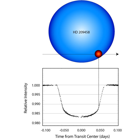
Nine extrasolar planets are known to transit their parent stars, but all of these planets have periods shorter than 5 days. They are frying beneath the brilliance of their parent stars. It would be nice to find a transiting planet with a longer period. Preferably, this would be a giant planet with towering thunderstorms and warm, drenching rains, and orbited by a habitable Earth-sized moon that we could detect with HST photometry.
This image from: http://www.nelsonhancockgallery.com/photography/AD.07.rain.lights-xl.jpg

Advanced observers can make the discovery of a transiting room-temperature Jupiter a reality by participating in the systemic team‘s distributed observing project: Transitsearch.org. A brief blurb on the transitsearch.org home page describes the basic strategy:

Transitsearch.org is a cooperative observational effort designed to allow experienced amateur astronomers and small college observatories to discover transiting extrasolar planets. In order to utilize the advantages of a network of small telescopes most effectively, our strategy is to observe known planet-bearing stars at the dates and times when transits are expected to occur.

At present, the majority of confirmed extrasolar planets have been discovered using the Doppler radial velocity technique (see the tutorials at www.oklo.org). The Doppler method, however, cannot determine the inclination of a planetary orbit to the line of sight from Earth. Therefore, each planet discovered by the Doppler method has an a-priori probability of transiting, which depends mainly on the orbital period of the planet. Short-period planets have relatively high transit probabilities, whereas long-period planets have low transit probabilities.

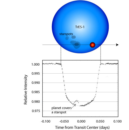
Transitsearch.org hasn’t found a new transiting planet. But if we can maintain the enthusiasm of the collaboration, then eventually it will. Every planet that is detected by the radial velocity technique has a finite a-priori probability of transiting. Hence we need to work systematically down through the list. Chances of success (among planets that have not yet been fully checked) range from a sporty 12.9% for HD 118203 “b” down to a depressingly low 0.1% for 55 Cancri “d” (for which our best-guess next opportunity to observe a transit center occurs, curiously enough, a week after the start of the next long count).

(more…)

GJ 876 — cracked with the console!

Users familiar with console tutorial #3 will have noticed that the self-consistent 2-planet fit to the remarkable multi-planet system orbiting GJ 876 is presented as a fait accompli. We are currently implementing an “epoch” slider for the console which will greatly smooth the transition from Keplerian to Newtonian fits for interacting systems, but amazingly, it turns out to be possible to obtain a competitive 3-planet fit to the Rivera et al (2005) GJ 876 data set using only the current version of the systemic console. This post gives the details, and gets a bit technical, so if you are interested in following it closely, we suggest that you first work through tutorials 1, 2, and 3.

Also, a cautionary remark. The 3-planet integrated fit requires patience. I was able to get the fit described below in about 2 hours on a machine with two 3.4 GHz Intel Xeon CPU’s (with hyperthreading turned on). Thus, I was able to use the other CPU’s to do other work. On single-core, single-processor machines, the systemic console will hog the CPU (unless it’s niced and put in the background).

In any case, here’s the 411:

(more…)

If the suit fits…

Five radial velocity datasets (published last year by Marcy et al. 2005) have just been added to the systemic console: HD 183263, HD 117207, HD 188015, HD 45350, and HD 99492. Each of these more-or-less sunlike stars is too faint to be seen with the naked eye, and each is accompanied by (at least) one detectable planet. The periods range from 17 days to several years. None of these planets were extraordinary enough to warrant much fanfare in the popular press. (Ten years ago, however, the announcement of 5 planets would have been front page news. Ahh, those were the days!)

When you use the console to obtain orbital fits to these systems, you’ll notice that several of the stars have a long-term radial velocity trend superimposed on the variations that arise from the much more readily detectable shorter-period planet. These velocity trends are likely caused by as-yet undetected massive planets lying further out in the systems, and as these stars are monitored over the long term, the orbits of these distant, frigid giants will gradually reveal themselves.

In the meantime, the residual velocity trends underscore an interesting general property of extrasolar planets. The presence of a known planet is the best indicator that a given star harbors detectable (but as-yet undetected) planetary companions. That is, if you want to find new planets, then look at stars that already have known planets. Indeed, six of the first twelve planet-bearing stars that were monitored for more than two years at Lick Observatory were subsequently been found to harbor additional bodies. This impressive planetary six-pack includes luminaries such as Upsilon Andromedae, 55 Cancri, and 47 UMa, in addition to the more pedestrian Tau Boo, HD 217107, and HD 38529. (See Fischer et al. 2001).

Planets at the AAS Meeting

Frequent visitors to oklo.org will have noticed a definite fall-off in the number of recent posts. This was a direct result of the start of the winter quarter here at UCSC, but now things are rolling, and the systemic team is working hard to prepare the next phase of the collaboration.

Last week was also the 207th meeting of the American Astronomical Association. I took a one-day trip to Washington in order to give a talk at Tuesday’s extrasolar planets session entitled, “From Hot Jupiters to Hot Earths“. I teach class on both Monday and Wednesday mornings, so the trip was more of a lightning raid.

a departure lounge at dulles international

I arrived at Dulles Airport at 6 am, after an overnight flight. My talk wasn’t finished, so I sat in an empty departure lounge for several hours and worked on the slides. By mid-morning, I realized that I had better head to the venue. I took a cab to the conference hotel, tapping on the laptop for most of the way.

Hundreds of astronomers were thronging in the hallways. I studied the posters that had been set up in a large exhibition hall, and then went to hear NASA Administrator Griffin give a keynote address, the gist of which was clearer than this snapshot (taken under low-light conditions).

NASA Administrator Griffin

Two of the things he said stuck in my mind.

Like it or not, NASA has been charged to fly to the moon for reasons that are completely divorced from astronomy, and this means that there will be opportunities to use a lunar platform for observations of extrasolar planets. Transit photometry of nearby stars, especially M-type stars, jumped to mind, but clearly, there is a serious opportunity right now to start thinking outside the box.

He also said that the primary education and outreach mission of NASA should be to inspire by doing “cool things”. I do remember watching the last Saturn V’s blast off for a lunar destination, and I remember, a few years later, learning in grade school science class, about the Space Shuttle, that “pickup truck into orbit”, and feeling distinctly less inspired. In the intervening years, my list of the coolest NASA things runs along the lines of, Voyager, HST, WMAP, Cassini-Huygens, and Spitzer. And there’s also the BPP project. (For more detail on interstellar missions, Paul Gilster’s Centauri Dreams is always the place to go).

Uh, my talk wasn’t all it could have been. In order to facilitate rapid transitions between the session speakers, everyone’s slides were uploaded to a central server. The server was running Windows, and all the Powerpoint presentations looked exactly like they were supposed to. Full screen ahead. As a Keynote user, however, my slides were in the form of .pdfs. They looked just fine in the speaker ready room, but then, when I stepped up to the podium, I was aghast to see that my .pdfs were displaying on only on a small portion of a screen containing an acrobat viewer, complete with a sneak “preview” and a sneak “review” of the next and previous slides. The resolution was too low to see any detail. Score one for Mr. Bill Gates.

For the record, though, here are the slides (full resolution .pdfs).

orbital

Let a pebble slip from your hand and it falls straight to the ground. Toss the pebble sideways, and it traces a parabolic arc through the air. Imagine throwing the pebble sideways with even more speed. It lands further away. Imagine throwing the pebble with such great velocity that the surface of the Earth begins to curve away beneath it as it falls. In the absence of air friction, a pebble thrown sideways with sufficient velocity will fall in such a way that the Earth curves continuously out from underneath. The pebble falls endlessly without ever touching the ground. It is in orbit.

Cassini view of Mimas, Dione and Rhea near the ring plane (credit: NASA/JPL)

The idea that an orbit is the state of a body in continual free-fall can be traced to the 1600s, and was first stated in print by Robert Hooke, whose paper entitled, “The Inflection of a Direct Motion into a Curve by a Supervening Attractive Principle” was read to the Royal Society on May 23rd 1666. Robert Hooke’s fame and reputation have spent the last three hundred and twenty years in Newton’s shadow, but he was a tremendously inventive scientist, and indeed, was one of the founders of what we now consider the scientific method. (See, for example, the recent Hooke biography, “The Forgotten Genius” by Stephen Inwood). Hooke, drawing on the earlier ideas of William Gilbert and Jeremiah Horrocks, and profiting from conversations with fellow Royal Society member Christopher Wren, realized that if the Sun exerts an attractive force on bodies in space, then “all the phenomena of the planets seem possible to be explained by the common principle of mechanic motions.” Hooke had an intuitive (but non-mathematical) understanding of the the orbit in the sense described in the paragraph that opens this post.

Robert Hooke was shouldered with a bewildering variety of interests and responsibilities. One of his many jobs was to produce weekly demonstrations for the entertainment and edification of the Royal Society. In order to illustrate his concept of the planetary orbit, he devised a demonstration that provided a suggestive analogy. A bob was placed on a long string pendulum. Tension from the string provided a central attractive force, and a sideways push provided the requisite tangential motion. When given a sideways push of exactly the correct speed, the bob would swing in a circle. When started at other speeds, it traced an elliptical path. With this simple device, Hooke was able to illustrate how an orbit is a compound of tangential motion and an attractive radial force.

Hooke then made the analogy more elaborate by attaching two bobs to the end of the string. Once set in motion, the two bobs would orbit each other, while their center of mass orbited the center of attraction:

compound pendulum

In 1670 , Hooke delivered a Cutler lecture at Gresham College, entitled, “An Attempt to Prove the Motion of the Earth by Observations”. The written version of this lecture contains three remarkable postulates, including, (1) a specification of the concept of universal gravitational attraction, that is, that mass attracts mass, (2) the assertion that all bodies “that are put into a direct and simple motion would continue to move in a straight line unless deflected”, and (3) the hypothesis that the attractive gravitational force falls off with distance. Taken together, these ideas are a remarkably correct qualitative formulation of the foundations of gravitational dynamics. Had Hooke been equipped with the mathematical skill to express his three ideas quantitatively, he would have gone very far indeed.

At the same time that Hooke was demonstrating his pendulum analogy to the Royal Society, Isaac Newton was nearing the close of his Anni Mirabiles. By 1666, Newton, who was working in total isolation, had found a quantitative model that explained the circular orbit, and also showed that gravity is manifested by an inverse square law of attraction.

I began to think of gravity extending to the orb of the Moon, & (having found out how to estimate the force with which a globe revolving within a sphere presses the surface of the sphere) from Kepler’s rule of the periodical times of the Planets being in sequialterate proportion of their distances from the center of their Orbs, I deduced that the forces which keep the Planets in their Orbs must [be] reciprocally as the squarres of their distances from the centers about which they revolve: & thereby compared the force requisite to keep the Moon in her Orb with the force of gravity at the surface of the earth, & found them to answer pretty nearly. (All of my Newton quotes are drawn from Richard Westfall’s “Never at Rest — A Biography of Isaac Newton“)

Here’s what Newton is saying. Kepler’s Third Law holds that the orbital period of a planet is proportional to the semi-major axis of its orbit to the 3/2 power, that is,

For the simplified case of a satellite in a circular orbit, the semi-major axis, a, is just the orbital radius, i.e. a=r. In Newton’s state of understanding in 1666, the “centrifugal” outward force an orbiting satellite must cancel the inward force exerted by gravitational attraction from the central body. The gravitational attraction is assumed to be spherically symmetric and to fall of with some power of the distance. That is,

where x needs to be determined. The fact that distance is rate multiplied by time implies that

and therefore

This means that

and if Kepler’s third law is to be satisfied, then x=2. Newton had realized that Kepler’s third law implies that gravity is an inverse-square force.

Newton had thus found a workable mathematical model for the circular orbit in 1666, but at that time, he was behind Hooke in terms of his intuitive understanding of the actual physical situation. Newton’s initial conception of the orbit was one of a mechanical equilibrium, in which an innate tendency to recede during circular motion is balanced by a gravitational attraction. In reality, Hooke’s concept of the orbit as the state of continual free-fall, a state of disequilibrium, is the correct notion.

On Nov. 24, 1679, Hooke, in his capacity as the secretary of the Royal Society, wrote a letter to Newton in order to solicit a discussion of orbital dynamics. Hooke was likely quite proud of his theories concerning orbital motion, and he may well have been eager to bring his ideas to Newton’s attention.

Let me know your thoughts of that of compounding the celestaill motions of the planets of a direct motion by the tangent and an attractive motion towards the centrall body.

Hooke had no way of knowing that Newton had already thought carefully about orbits. It is likely that as soon as Newton saw Hooke’s phrase, he immediately saw that it represented an improved qualitative conception of orbital motion. He quickly wrote back to Hooke, and politely declined the offer of an extended dialog. He, was, he said, too busy with other studies.

And having thus shook hands with Philosophy, & being also at present taken of with other business, I hope it will not be interpreted out of any unkindness to you or the R. Society that I am backward in engaging my self in these matters…

Nevertheless, the correspondence between the two continued through several more letters. By January 1680, Hooke had managed to guess (on the basis of two incorrect arguments that combine by chance to give a correct formula) that the gravitational force obeys an inverse square law. What he could not prove, however, was what the general path of an orbiting planet is an ellipse (that is, he could not go beyond the special case of the circular orbit). The fact that the planetary orbits have elliptical figures was then known empirically from Kepler’s First Law, which states that planetary orbits are ellipses with the Sun at one focus.

On January 6th, 1680, Hooke took the liberty of informing Newton of the inverse square law, “My supposition is that the Attraction always is in a duplicate proportion to the Distance from the Center Reciprocall…”, and in a letter on the 17th of January, he further urged Newton to find the general mathematical description of a planetary orbit,

I doubt not but that by your excellent method you will easily find out what that Curve must be, and its proprietys, and suggest a physicall Reason of this proportion.

Hooke’s letters of November through January of 1679-80 seem to have greatly annoyed Newton. With his formidable intuition and dismal mathematical skills, Hooke was steadily blundering toward the pedestal where he could claim the renown of explaining the “System of the World”. Without informing Hooke, Newton carried out (in early 1680) a marvelous derivation that showed that the path of a planet is an ellipse, and simultaneously proved Kepler’s Second Law, which states that the radius vector of a planet sweeps out equal areas in equal times, and which is a statement of the principle of the conservation of angular momentum.

Years later, soon after the appearance of the Principia, when Hooke claimed that Newton had plagiarized his ideas, Newton lashed out at Hooke in a letter to Edmund Halley:

Should a man who thinks himself knowing, & loves to shew it in correcting & instructing others, come to you when you are busy, & notwithstanding your excuse, press discourses upon you & through his own mistakes correct you & multiply discourses & then make use of it, to boast that he taught you all he spake and oblige you to acknoledge it & cry out injury and injustice if you do not, I beleive you would think him a man of a strange unsociable temper.

Robert Hooke, that man of strange unsociable temper, is nevertheless a man after my own heart. Newton is so far out on the curve that I can’t relate to him at all. I have no concept of how his mind operated, but Hooke, Hooke would be a fantastic person to have a beer with. I can appreciate the way he thought by analogy. I greatly admire his demonstrations, even if they aren’t fully rigorously correct.

With Hooke’s approach in mind, let’s look at some elliptical orbits. When an ellipse has zero eccentricity, the two foci come together, and the ellipse is a circle. A planet on a circular orbit travels at constant speed, and its positions at a hundred equally spaced time intervals are equally spaced:

e=0 ellipse

When the eccentricity reaches 0.1, the orbit looks very much like a shifted circle. When the planet is closest to the Sun (the point known as perihelion), it is moving faster. If you look carefully, you can see that the dots are spaced just a bit more sparsely on the right side than on the left. The e=0.1 orbit just below is very similar to the orbit of Mars, which has an eccentricity e=0.0935. In all of the following figures, the e=0 circular orbit is also shown for comparison:

e=0 ellipse

Among the eight major planets in our Solar System, Mercury, with e=0.205, has the most eccentric figure. Mercury’s orbit is almost identical to the orbit in this plot, which has e=0.20:

e=0 ellipse

Planets “c” and “d” of the Upsilon Andromedae system have eccentricities of e=0.27 and e=0.28 respectively. Their orbital figures are quite close to this orbit, which has e=0.3:

e=0 ellipse

70 Vir b was one of the first extrasolar planets to be discovered. It has a very well defined orbit with e=0.4:

e=0 ellipse

When e=0.5, it’s impossible to mistake the ellipse for an off-center circle. The extrasolar planet GJ 3021 b has an eccentricity e=0.511, which is close to e=0.5:

e=0 ellipse

At an eccentricity e=0.6, the brevity of the periastron swing is highly pronounced:

e=0 ellipse

When e=0.7, the planet is 5.667 times closer to the star at periastron than at apastron.

e=0 ellipse

e=0 ellipse

e=0 ellipse

The extrasolar planet with the highest known eccentricity, HD 80606 b, has an 111 day orbital period and e=.938. See my article on this strange world posted last month. Because it dives in so close to its parent star, HD 80606 b is an interesting transit candidate, but a transitsearch.org campaign carried out last year did not detect transits. We’ll try again this year during the upcoming transit opportunities.

Do you give talks on extrasolar planets? High-resolution .pdf files of the above orbital plots are free here for the taking: e=0.0, e=0.10, e=0.20, e=0.30, e=0.40, e=0.50, e=0.60, e=0.70, e=0.80, e=0.90.