55’s the limit

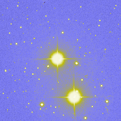
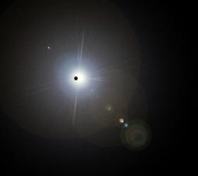
55 Cancri is an ordinary nearby star, barely visible to the naked eye. Through a modest telescope (or, more practically, with the use of the Goddard Skyview) one sees that it is actually a binary pair.

Goddard Skyview Image of 55 Cancri

55 Cancri “A” (the bright star in the middle of the above photo) harbors an extraordinary planetary system. Indeed, it was the subtlety and the depth of the 55 Cancri radial velocity data set that motivated us to develop the systemic console. The fact that the 55 Cancri system continues to defy easy categorization gives us confidence that the systemic collaboration will be a worthwhile project.

Where to begin?

Click on the system menu on the console, scroll down, and select 55 Cancri. (If you’re unfamiliar with the console, and if you’re the methodical type, there are three tutorials available on the menu bar to the right. Otherwise, just follow along!) The published radial data for 55 Cancri now appears in the main console window. The sweeping spray of points, with its curiously non-uniform distribution, contains a fascinating narrative in its own right.

The very first point in the data set has a timestamp of JD 2447578.73 A Julian Date Converter tells us that this was 9:31 PM on Monday Feb. 20, 1989 (Pacific Standard Time). The observation was obtained by Geoff Marcy at the Shane 3-meter telescope at Lick Observatory on Mt. Hamilton, and the velocity error is 9.7 m/s. Back in 1989, Geoff and his colleague Paul Butler were laboring to improve their iodine cell technique, and were struggling to get enough telescope time to adequately track the motion of about 70 nearby solar type stars with the eventual hope of detecting giant planets.

The first 10 radial velocity points were obtained at a rate of 1 to 3 per year. With hindsight, it is easy to see that these 10 points are ample cause for a planet-hunter to be optimistic. The radial velocity variation in the first 10 points spans more than 100 meters per second, suggesting a signal with a signal-to-noise of at least five. The periodogram of these ten points shows a strong peak at 14.65 days, indicating that the data could be explained by a planet with 80% of Jupiter’s mass, circling on an orbit lasting just over two weeks.

Today, if such a planet were discovered, the announcement would not make the news, and the major excitement would be among amateur transit hunters, who would likely have a new high-priority follow-up candidate with a ~5% transit probability. (A two-week period is right at the borderline where transits can be reliably confirmed or ruled out by the photometric collaborators working with the RV-discovery teams prior to announcement of the planet).

In 1993, however, nobody was expecting to find Jovian planets in 14-day orbits. Conventional wisdom at the time was informed by the architecture of our own solar system, and held that gas giant planets should be found beyond the so-called snowline (located at r=4-5 AU) of the protostellar disk. Although the theory of orbital migration had been studied in considerable detail, nobody had proposed that giant planets might regularly spiral in and then be marooned on very short-period orbits. I don’t know whether Geoff and Paul even considered the possibility that the 14.65 day peak in their data was real. If they saw the peak, it is more likely that they would have ascribed it to an alias, an artifact of their uneven hard-won sampling.

During 1994, the velocities suddenly started to trend upward. This would have seemed rather disconcerting, and may even have raised alarm. Was some unaccounted-for instrumental or astrophysical process affecting the newer radial velocity data? Certainly, at the end of 1994, the case for a planet orbiting 55 Cancri would have been weaker than it had been a year earlier.

Nevertheless, the 55 Cancri campaign was at an important turning point. The last measurement of 1994 (JD 2449793.80) has a remarkably lower error (3.3 m/s) than any of the earlier radial velocities. In November of 1994, the Schmidt camera optics on the “Hamilton” spectograph at Lick Observatory had been upgraded, and the resulting improvement effectively tripled the intrinsic resolution to which the spectral lines could be discerned. With the ability to measure radial velocities to a precision of 3 m/s, the planet search had suddenly entered an entirely new realm. When one is in the business of detecting Jupiters, a velocity measurement with 3 m/s precision is literally 10 times as valuable as a velocity with 10 m/s precision.

In October 1995, Mayor and Queloz announced their discovery of a Jupiter-like planet in a 4.5 day orbit around the nearby star 51 Peg. Due to a catalog error that misclassified 51 Peg as a subgiant, it had not been included in Geoff and Paul’s survey, but they were able to rapidly confirm the Swiss discovery.

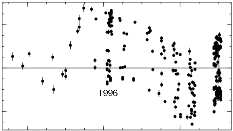
All at once, the idea of a gas giant with a 2-week orbit was no longer outlandish at all. The telescopes on Mt. Hamilton, which had been slipping inexorably in worldwide prestige as larger telescopes were built on higher mountains, were suddenly at the forefront of relevance. The Lick 3-meter telescope-iodine-cell-spectrograph combination was the best instrument in the world for obtaining precision doppler velocities of bright stars such as 55 Cancri. Extrasolar planets were front page news. Alotments of telescope time increased dramatically. In the six months running from December 1995 through May 1996, 55 Cancri was observed 41 times at Lick. This drastic increase in the cadence of observations is easily visible in the radial data:

1996 RVs

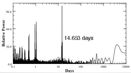
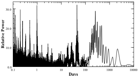
With the 41 high-quality observations, the presence of the 14.65 day planet was obvious in the power spectrum.

RV powerspectrum

In October 1996, Paul, Geoff, and several other collaborators announced the discovery of the 14.65 day planet, and in January 1997, they published the discovery in a now classic paper that also introduced the world to the inner planetary companions of Tau Bootes and Upsilon Andromedae.

With eight years of data, it was clear that other bodies were present in the system. In the discovery paper, Butler et al. wrote:

The residuals exhibit a long-term trend, starting at -80 m/s in 1989 and climbing to +10 m s-1 by 1994 (the velocity zero point is arbitrary). The velocities appeared to decline toward 0 m s/1 during the past year, although at least another year of data will be required for confirmation. This trend and the possible curvature in the velocity residuals are consistent with a second companion orbiting HR 3522 [aka 55 Cancri] with a period P > 8 yr and M sin i > 5MJUP.

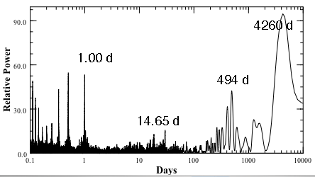
This speculation proved to be correct. Use the console to get a best-fit for the 14.65 day planet, and compute the periodogram of the residuals to the fit:

RV residuals powerspectrum

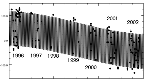
The strongest remaining peak is at 4260 days, corresponding to an 11.7 year orbit (very similar to Jupiter’s 11.8 year orbital period). Keeping the orbits circular, use the “polish” button to produce a Levenberg-Marquardt optimized fit. Zoom in and scroll to show the time interval between 1996 and 2002. The gaps each year when the star is behind the Sun as seen from Earth are easily visible:

Lick RVs 1996-2002

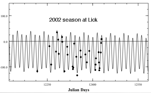
The two planet system does quite a reasonable (but by no means perfect) job of reproducing the observed radial velocities. After the announcement of the first planet at the end of 1996, interest in the star died down to some degree. The number of target stars being observed at Lick was being increased as Debra Fischer stepped in to manage the Lick Survey, and other systems, especially Upsilon Andromedae, were clamoring for telescope time. During the 1998 season, 55 Cancri was observed only twice. By 1999, however, the Upsilon Andromedae system had been sorted out, and renewed attention was focused on 55 Cancri. During 2000 and 2001, it became clear that the system likely contained at least three planets. With the 14.65 and (in my fit) 5812 day planets removed from the radial velocity curve, the residuals periodogram shows a peak at 44.3 days:

residuals of the residuals

The signal from the 44.3 day planet is not as strong as for the other two planets, but a large number of velocities from 2002 seemed to clinch the case for this third planet:

residuals of the residuals

Use the console to optimize the three planet fit using circular Keplerian orbits. When I do this, the chi-square statistic is reduced to 6.4, and the rms scatter is 12.5 m/s. The fit is still not perfect. Either the planets are eccentric, or there are additional planets in the system.

Why does HD 209458 b wear an XXL?

extrasolar planetary transit

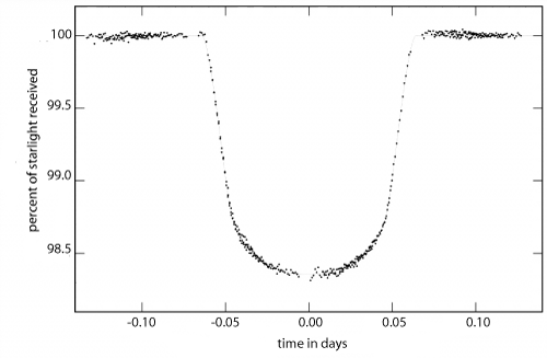
In 1999, the sun-like star HD 209458 was discovered to harbor a transiting planet on a 3.52 day orbit. This was a big deal. The recurring occultations permitted, for the first time, an accurate measurement of both the radius and the mass of an extrasolar planet, and there have been a huge number of follow-up observations of the transits using a variety of telescopes and techniques. The most impressive result came from Brown et al. (2001), who used the (now defunct) STIS instrument on the Hubble Space Telescope to obtain a photometric light curve that has precision of about one part in ten thousand per 80-second sample:

extrasolar planetary transit

The plot above can be found in the Astrophysical Journal , or, alternately, the paper containing the plot is available for free at the arXiv preprint server. A careful analysis of the photometric curve and the radial velocity data (which can be explored using the systemic console), combined with estimates for the size, mass and other properties of the parent star, indicates that the planet, HD 209458 “b”, has a radius about 1.35 times larger than the radius of Jupiter, and a mass of 0.69 times Jupiter’s mass. The temperature on the surface of the planet should be a toasty ~1200 K.

Various teams of scientists, including a group led by Peter Bodenheimer here at Santa Cruz, and independent groups led by Tristan Guillot and Gilles Chabrier in France, and Adam Burrows’ group in Arizona have all developed detailed computer programs that can predict how planets respond when placed in different physical environments. Everybody agrees that a gas giant planet with a standard hydrogen-helium composition and the mass and surface temperature of HD 209458 b should have a radius (corresponding to the 1-Atm pressure level) that is about 5-10% larger than Jupiter. The observed size of the planet is thus far out of agreement with the theoretical models. The planet is too large!

As soon the size problem became clear, a number of explanations for HD 209458 b’s large radius were put forward. The Burrows group (2003) pointed out that the planet may appear large during the transit because we are looking obliquely through long path lengths in the planetary atmosphere. Tristan Guillot and Adam Showman (2002) suggested that the ferocious winds on the planetary surface are transferring energy into the deeper layers of the planet, and that this extra source of energy is enough to bloat the planet to its observed size. These two phenomena don’t require anything special about HD 209458 b, and so both hypotheses predict that other planets with similar masses and temperatures should have similarly inflated radii. This doesn’t seem to be the case, however. In August 2004, a transiting planet of very similar mass and temperature was found in transit around an 11.8 magnitude star known as Tres-1 (Alonso et al. 2004). This planet has exactly the size (~1.05 Jupiter radii) predicted by the baseline theories. It thus appears that there is something unusual about HD 209458 b.

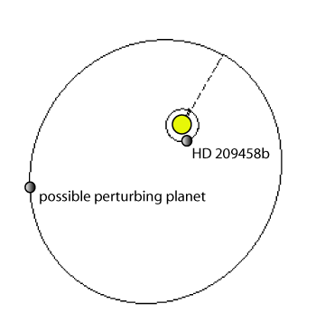
One intriguing possibility, suggested by Peter Bodenheimer, Doug Lin and Rosemary Mardling in 2001, is that another planet exists further out in the HD 209458 system. This planet would be exerting gravitational perturbations on HD 209458 b, which would cause its orbit to maintain a small eccentricity. If a planet like HD 209458 is in an eccentric (non-circular) orbit, then it experiences significant tidal stretching and squeezing which generate heat in the planetary interior. In a follow-up paper published in 2003, Bodenheimer et al. calculated that an orbital eccentricity, e=0.03 would likely be sufficient to generate enough tidal heating to inflate HD 209458 b to the observed size.

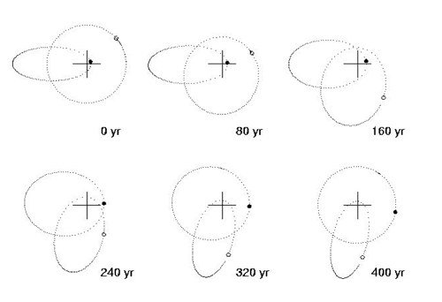
At that time, there were only 30 high-precision radial velocity measurements of HD 209458, and it was easily possible to find 2-planet fits to the radial velocity data which had (1) a small non-zero eccentricity for HD 209458 b, as well as (2) a second planet with a period of order 80 days, and a mass of ~0.12 Jupiter Masses. In the following diagram, the orbits are to scale, but the star and especially the planets are grossly too big.

a perturbing body

Over the past two years, the California-Carnegie Planet Search Team used the Keck telescope to obtain a number of additional radial velocity measurements of HD 209458, and these have been published in a new paper. The full set of (out-of-transit) measurements have been loaded into the system menu of the systemic console. In our paper, our conclusion was that HD 209458 b is likely the only RV-detectable planet in the system, and that its orbit is most likely circular (more on this in a future post). See, however, if you can use the console to find viable 2-planet fits that have the correct period for the inner planet P=3.52474541 d, and which have a required RMS jitter for the star of less than 5 m/s. (Technically, you should also apply a simultaneous constraint on Mean Anomaly and eccentricity that arises because the time of central transit is known very accurately, but the console doesn’t yet have this capability. If you find a good fit, and post it here, we can likely fold in the additional timing constraint without greatly changing the basic orbital parameters).

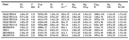
The number of known transiting planets has been increasing steadily, and the total now stands at nine. Using the results of Peter Bodenheimer’s planetary structure code, we can compare the planets predicted sizes with their observed sizes:

the properties of the known transiting planets

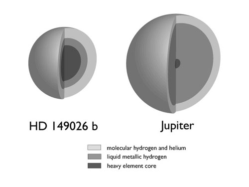
(Here’s a larger-size .pdf of the above table, which will appear in an upcoming PPV review article). Three of the planets in the table, HD 209458b, HD 149026b, and HD 189733b, have radii that do not agree at all with the predictions. HD 209458b (and to a slightly lesser extent) HD 189733b are both larger than predicted, whereas HD 149026b is too small, likely because it has a huge rocky core:

a size comparison

These discrepancies indicate that the bulk properties of the transiting planets must depend significantly on factors other than their mass and estimated effective temperatures. Like the planets of our solar system, the extrasolar planets are imbued with interesting individual personalities.

fresh extrasolar planets

fresh extrasolar planets

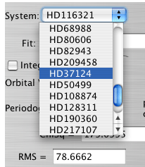
In a recent article appearing in the Astrophysical Journal, Vogt et al. (2005) published radial velocity data for six stars that appear to harbor multiple low-mass companions. The data for all six stars (HD 37124, HD 50499, HD 108874, HD 128311, HD 190360, and HD 217107) have been added to the system menu of the Systemic Console:

new systems in the console

If you’ve worked through the console tutorials 1, 2, and 3, take a crack at using the console to fit these systems. HD 37124, in particular, is open to several different stable 3-planet configurations. In my current personal favorite fit, three very nearly equal-mass planets are caught up in an endless (or at least multi-billion year) cycle of rub-a-dub-dub. An .mpg animation of the long-term dynamical evolution of the orbits is here. Because the planets in this particular fit are fairly widely spaced, the motion is quite well described by second-order secular theory.

i wear my sunglasses at night

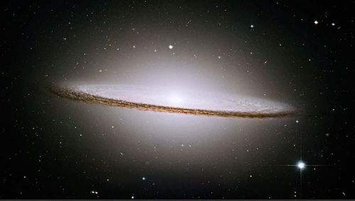
Of all the photographs that our robot emissaries have radioed back to Earth, my vote for the most stunning is the Hubble ACS image of the “Sombrero Galaxy”, M104. The glow of its halo makes the the idea of 100 billion stars seem comprehensible.

HST ACS mosaic of M104

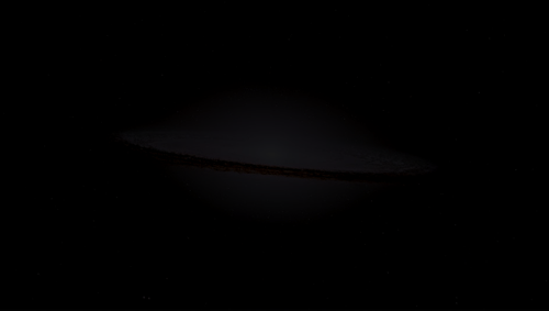
It’s important to remember, however, that the Hubble image is actually a long CCD time-exposure to light gathered by a 240 cm mirror. If you could be somehow transported to a location in space where M104 looms large in the sky, you would see that HST imparts a severely inflated expectation. From a distance, say, of 300,000 light years, M104 would be so dim that you would see only a faintly ominous, faintly glowing flying saucer.

Approximate naked-eye view of M104 from ~300,000 light years distance

Indeed, the great Andromeda Galaxy, M31, subtends an angle larger than the full Moon in the sky, and it is literally almost directly overhead right now (9:36 PM, Dec 3, latitude 36.97 deg N). The storms from earlier this week have blown through. The sky sparkles with brilliant clarity. Yet when I step outside and look up, I can’t see the Andromeda Galaxy at all. It’s too faint. In a 1:10,000,000,000,000 scale model of M31, the stars are like fine grains of sand separated by miles. Our Galaxy, the Andromeda Galaxy, and the Sombrero Galaxy are all essentially just empty space. To zeroth, to first, to second approximation, a galaxy is nothing at all.

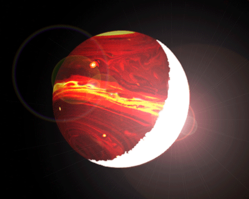
A Hot Jupiter, on the other hand, seen at similar angular size, is undeniably impressive.

HD 149026 b in the crescent phase

The dayside, blindingly illuminated by the scorching proximity of the star, is roughly 500 times brighter than desert sand dunes on a midsummer day. In order to look at the illuminated side of the planet at all, you need extremely dark wraparound sunglasses, or better yet, an eyeshield made from #10 welders glass (where #14 welder’s glass is recommended for those who stare at the sun).

With the brilliance of the dayside cut to a manageable level, what would you see? The majority of the light coming from the planet is simply reflected starlight. If the planet uniformly reflects the light that strikes it, then you simply see a blank white surface if the parent star is similar to the Sun, and a yellow-orange to orange-red expanse if the parent star is a cooler K-type or M-type dwarf star.

The gases that make up the outer layers of the planet do not reflect all frequencies of light equally, however. The air of the outer layers of a hot Jupiter is a scaldingly toxic witches brew of hydrogen, helium, steam, methane, ammonia, cyanide, acetylene, hydrogen sulfide, soot, and a whole host of other hardy, reactive, and generally unpleasant compounds.

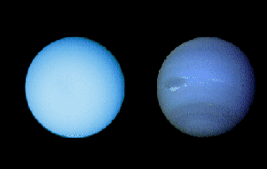
In our solar system, for example, Uranus and Neptune have distinctive blue-green casts because at the level in their atmospheres where light is primarily reflected, the ambient methane gas is highly effective at absorbing red frequencies. The originally white sunlight is reflected with a blue-green hue by the selective removal of red.

Uranus and Neptune (from Voyager II)

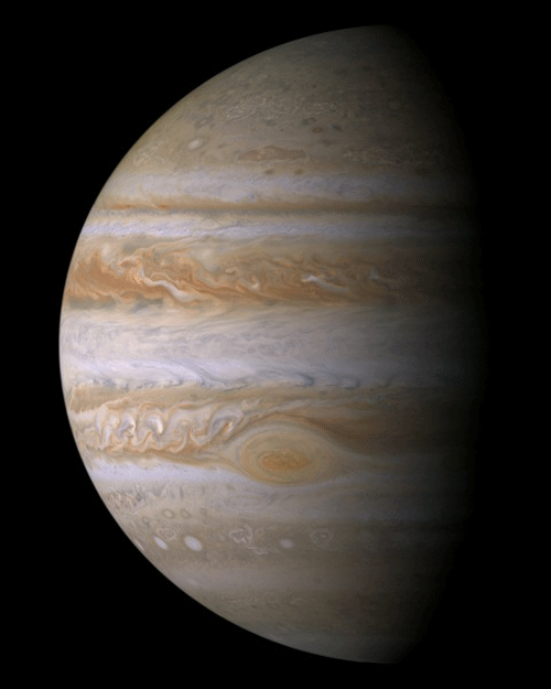
The photo (mosaic) below was obtained by the Cassini spacecraft as it was flung past Jupiter on its way to Saturn. The images were processed to give the same view that the naked eye would see. Jupiter reflects an enormous amount of detail from its cloudy face.

True-color Cassini mosaic of Jupiter

Across the swathes of Jupiter where the visible clouds tower to great heights, the eye sees regions that are frigid, eighty degrees colder than the depths of an Antarctic winter (-200 F). In such a cold environment, icy compounds of Ammonia are stable, and their presence lends the clouds a reddish hue. Jupiter’s Great Red Spot is an example of just such a topographic high.

On other regions of Jupiter’s visible surface, the atmosphere is transparent to greater depths. As on Earth, where clear skies are associated with dry air, so too on Jupiter. When we look down into the drier Jovian regions, we see to lower lying decks of cloud where the temperature is about the same as a chilly Arctic night. Here, the chemistry in the clouds causes their color to tend toward lighter shades, whites, beiges, ochers.

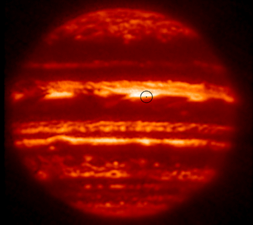
Like any non-transparent object, Jupiter glows with its own radiation. Because the outer layers of Jupiter are so cold, this intrinsic light lies in the infrared. Seen with an infrared detector (such as this view made at 5 microns with the NASA IRTF) Jupiter is a dramatic sight.

IRTF 5 micron image of Jupiter

In the rattlesnakes-eye view, the Red Spot forms an oval of relative darkness. The high clouds act like a blanket that blocks the warmer underlying layers from view. In the infrared, the dry areas, where we see the deepest, glow the brightest. In an ironic twist of fate, the Galileo atmospheric probe parachuted into one of the driest regions of the Jovian atmosphere, a so-called 5 micron hot spot (circled in the image above).

On a hot Jupiter, the surface gas is heated to temperatures in the 1000-1500 K range on the dayside. Computer simulations show that winds of hellacious strength tear continually around the planet, carrying heat from the dayside and disgorging it into the night. The atmosphere on nightside glows brilliantly. Turbulent brick-red whorls merge into fiery tendrils of orange braided with dazzling white.

A most eccentric character

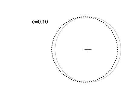
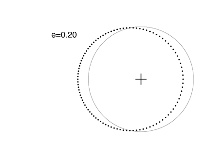
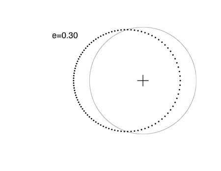
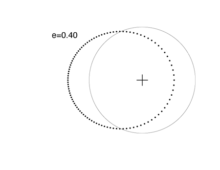
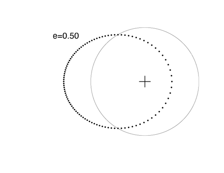
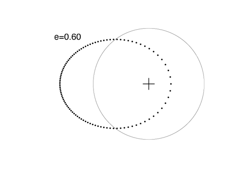
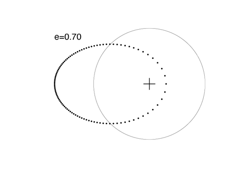
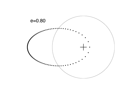
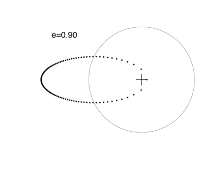
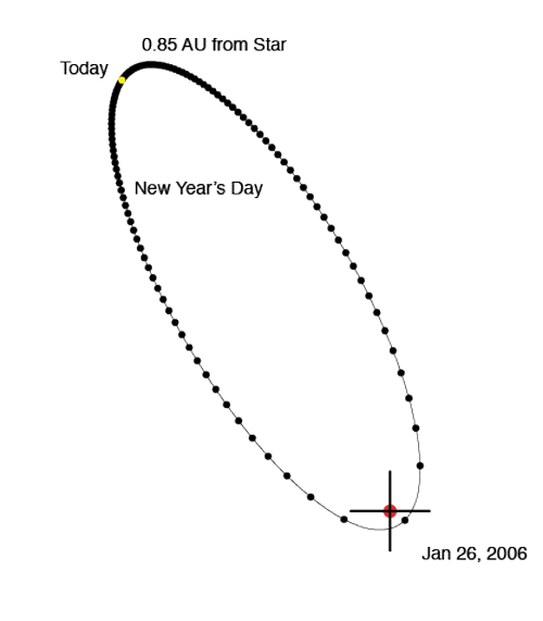
Of all the known extrasolar planets, HD 80606b — in both the technical and the colloquial sense — is the most eccentric. This world has at least five times the mass of Jupiter, and it circles its parent star on an extremely elongated 111.4 day orbit:

planetary orbit for HD 80606 b

Today (as seen from Earth!) HD 80606b is still near the far point of its orbit, at a distance of about 0.85 AU from the central star. The temperature in the upper atmospheric layers of the night-side has possibly dipped low enough so that torrential rains and violent thunderstorms are rumbling across its vast billowing horizons. During the rest of December and through most of January, the planet will fall in almost the full distance to the star, eventually swooping within 6 stellar radii as it whips through periastron. On January 26th, at the moment of closest approach, the temperature at the cloud tops will exceed 1000 Kelvin. The auroral displays will be dramatic beyond compare, and indeed, during the days to either side of periastron passage, it might be worth tuning in to the planet on the decameter band.

The discovery of the planet and its orbital solution were announced by the Geneva Observatory Planet Search Team in an April 04, 2001 ESO press release, and the radial velocities have since been made publicly available (right on!) at the CDS repository (see Naef et al 2001). You can therefore use the systemic console to fit this system and examine how radial velocity curves behave for extremely eccentric orbits.

The star HD 80606 is accompanied by a visual binary companion, HD 80607. The projected separation of the two stars is 2000 AU (fifty times the Sun-Pluto distance). When the HD 80606 b travels through the segment of its orbit that lies between the two stars, the night-side cloud tops of the planet are lit by the distant binary companion to ambient brightness that is very similar to a fully moonlit night on Earth. The two stars have similar masses, sizes, and temperatures to the Sun, but, like many of hosts of short-period massive planets, they are enriched in “metals” (gold, chromium, iron, carbon, oxygen, etc. etc.) by a factor of more than two relative to the solar value.

How did the planet get into its weird orbit?

Wu and Murray (2003) have suggested that HD 80606b’s extreme eccentricity is the result of a three-body interaction known as the “Kozai effect” between the planet and the two stars.

The next big thing

We know that planets aren’t rare, and by now, with the tally over at the extrasolar planet encyclopedia poised to blast past 200, the announcement of a newly discovered run-of-the-mill Jupiter-sized planet barely raises the collective eyebrow.

The headline that everyone is anticipating is the discovery, or better yet, the characterization of a truly habitable world — a wet, Earth-sized terrestrial planet orbiting in the habitable zone of a nearby star. Who is going to get to this news first, and when?

299 million dollars of smart money says that Kepler, a NASA-funded Discovery mission currently scheduled for launch in June 2008, will take the honors. The Kepler spacecraft will fly in an Earth-trailing 377.5 day orbit, and will employ a 1-meter telescope to stare continuously (for at least four years straight) at a patchwork of 21 five-square-degree fields of the Milky Way in the direction of the constellation Cygnus. Every 15 minutes, the spacecraft will produce integrated photometric brightness measurements for ~100,000 stars, and for most of these stars, the photometric accuracy will be better than one part in 10,000. These specs should allow Kepler to detect transits of Earth-sized planets in front of Solar-type stars.
Kepler has a dedicated team, a solid strategy, and more than a decade of development work completed. It’s definitely going to be tough to cut ahead of Bill Borucki in line. Does anyone else stand a chance?

Practitioners of the microlensing technique have a reasonably good shot at detecting an Earth-mass planet before Kepler, but microlensing-detected planets are maddeningly ephemeral. There are no satisfying possibilities for follow-up and characterization. Doppler RV has been making tremendous progress in detecting ever-lower mass planets, but it seems a stretch that (even with sub-1 meter per second precision) the RV teams will uncover a truly habitable world prior to Kepler, although they may well detect a hot Earth-mass planet.

There is one possibility, however, whereby just about anyone could detect a habitable planet (1) from the ground, (2) within a year, and (3) on the cheap. Stay tuned…

Now fielding three tutorials

Three detailed console tutorials have recently been developed, and are now online at oklo.org.

Tutorial #1 steps through the basic features of the console, using the published radial velocity data-set for the Jupiter-like planet orbiting HD 4208.


Tutorial #2
takes a more detailed look at the console, and shows how to use periodograms and multiple-planet fitting to recover the three planetary companions (the so-called Fourpiter, Twopiter, and Dinky) orbiting Upsilon Andromedae.


Tutorial #3
tackles the tough problem of multiple-planet fitting in the presence of planet-planet interactions, and uses the console to explore the remarkable, recently published Gl 876 data set.

The console has landed.

After more than a year of development work, the beta version of the systemic console java applet is now up and working at oklo.org. Hats off to Aaron Wolf for coding it into reality.

In a series of posts, we will look in detail at the organization, operation, and features contained in the console. For now, however, rev up your G4s and your G5s, take it for a spin, and let us know how it works for you.

The current location for the console is:

www.oklo.org/SystemicBeta/SystemicBeta.html.

It’s also accesible from the menu bar to the right. At the moment it has been tested only with Safari 2.0.2 running on OSX 10.4.3. Firefox 1.0.6 still seems to have issues with the applet. We’ll resolve these first, and then (with CDR Paul Shankland leading the charge) we’ll move on to thwart Bill Gates’ best attempts to protect the MS Explorer user base from Systemic’s seductive charms…

All hands on deck (GJ 876)

nsf illustration of GJ 876 d

Paul Shankland has been visiting Santa Cruz this week, and everyone agrees that it’s about time to get the GJ 876 transit situation sewed up once and for all. Aquarius is still up in the early evening, and a planet “c” transit opportunity is bearing down with 30.1 day semi-clockwork precision. So out went the following alert to the transitsearch.org e-mail list:

Thursday Afternoon, Nov. 17, 2005

Dear Transitsearch Observers,

We’d like to alert you to an opportunity to check the GJ 876 system for planetary transits. Photometry is desired during a twelve-hour window centered on JD2453693.491 (Friday Nov. 18, 23:47 UT).

As you have likely heard, the GJ 876 system was recently found to harbor a low-mass (7.5 Earth Mass) planet on a 1.94 day orbit. The new planet is referred to (rather prosaically) as GJ 876 “d”, and is the third planet detected in the GJ 876 system. The discovery paper is scheduled for an upcoming issue of the Astrophysical Journal, and is also available on the astro-ph preprint server: http://arxiv.org/abs/astro-ph/0510508

Sadly, transits for planet “d” have been ruled out to high confidence.

As a result, however, of (1) inclusion of the third planet in the dynamical model for the system, and (2) a large number of new high-precision radial velocities, Eugenio Rivera has produced new transit ephemeris predictions for the outer two planets in the GJ 876 system. These differ by several hours from the dynamical predictions that are currently posted on the transitsearch.org candidates site, e.g.:

http://www.ucolick.org/~laugh/GJ876____c.transits.txt

We’re working through an extensive analysis which shows that neither “b” nor “c” is transiting, but this analysis is nevertheless in great need of observational verification. There is a conflict between dynamical fits to the radial velocities (which indicate that the system is inclined by 50 degrees to the plane of the sky) and the results of Benedict et al (2002, ApJL 581, 115), who used HST to get astrometric measurements that suggest a nearly edge-on configuration.

We’d thus like to request photometry of the star to six hours on either side of JD2453693.491 (Friday Nov. 18, 23:47 UT).

Information regarding observing GJ 876 and photometry submission instructions are at:

http://www.aavso.org/news/ilaqr.shtml

Additional background is on the transitsearch GJ 876 results page:

http://www.ucolick.org/%7elaugh/GJ876____c.results.html

Note that this page states that the photometric campaign is over, but the new dynamical model indicates that more photometry is desirable.

Other observing opportunities are (were) as follows:

For planet c (the middle one):

predicted central transit (UT)
————————————
2005 Aug. 20 15:40
2005 Sep. 19 18:41
2005 Oct. 19 20:53
2005 Nov. 18 23:47
2005 Dec. 19 01:36

For planet b (the outer one):
————————–
2005 Aug. 22 17:28
2005 Oct. 22 17:34
2005 Dec. 22 18:05

Finally, we’d like to thank everyone for being patient over the 8 months, during which we have not been running coordinated campaigns. With Shankland of USNO “on the bridge”, we’re now ramping up for a more active phase. Stay tuned!

The music of the spheres (sounds terrible)

After using the console for a while, you’ll notice that it’s often easy to find a reasonably good (say, chi-square of 3-5) multiple-planet fit to a given radial velocity data set. This rule of thumb tends to be especially true if you allow the planets to have large eccentricities. But how does one know whether the fit is likely to be correct?

This is one of the questions that the systemic simulation is designed to answer.

Most of the time, however, if a fit contains large enough eccentricities for the planet orbits to cross, then the trial system will be dynamically unstable. That is, the planets in the model will suffer a close encounter, which is generally followed (or directly accompanied) by a disaster. The planets collide, or one or more of them is ejected, or one of them is thrown into the central star.

While it is certainly true that such catastrophes have been reasonably common throughout galactic history, it is exceedingly unlikely that any particular planetary system that we observe will be on the verge of a dramatic instability. The stars that can be observed using the Doppler radial velocity method are billions of years old. If a star had an unstable planetary system, it is likely that the instability either occurred long ago, or that won’t happen for a long time to come.

As a result, an important requirement for any radial velocity fit is that it correspond to a dynamically stable system. Traditionally, this can be checked either by integrating the system forward in time, or by applying a technique which checks for the presence of chaos in the orbits. (Indeed, all of the planetary systems that underlie the systemic database have been integrated for one million orbits prior to being “observed”. These pre-integrations establish a strong likelihood of short-term dynamical stability for all the systemic systems.)

Here’s an idea that sounds possibly promising. If the radial velocity waveform of a planetary system is converted into an audio signal, is it possible for the human ear to rapidly detect whether a system is likely to be unstable? To test this, we’re working on bringing an audio generator into the systemic console.

More generally, what do the extrasolar planetary radial velocity reflex waveforms sound like? The short answer is, they sound terrible. There are interesting reasons for this, which we’ll pick up in a future post. For now, have a listen to these .wav’s (created by Aaron Wolf) of two of the best-known multiple planet systems: GJ 876 and Upsilon Andromedae

And try to listen for the (heavily processed voice of the better-voice-of-the-two GJ876 in the forthcoming James Alley Remix).

Hello world.

What is systemic?

Systemic is a public research collaboration. Systemic’s goal is to obtain a better understanding of the census of planets in the galaxy.

The systemic blog, hosted by oklo.org, provides a framework for updates and information relating to the collaboration. It also serves as an online forum for discussion of extrasolar planets.