Users familiar with console tutorial #3 will have noticed that the self-consistent 2-planet fit to the remarkable multi-planet system orbiting GJ 876 is presented as a fait accompli. We are currently implementing an “epoch” slider for the console which will greatly smooth the transition from Keplerian to Newtonian fits for interacting systems, but amazingly, it turns out to be possible to obtain a competitive 3-planet fit to the Rivera et al (2005) GJ 876 data set using only the current version of the systemic console. This post gives the details, and gets a bit technical, so if you are interested in following it closely, we suggest that you first work through tutorials 1, 2, and 3.

Also, a cautionary remark. The 3-planet integrated fit requires patience. I was able to get the fit described below in about 2 hours on a machine with two 3.4 GHz Intel Xeon CPU’s (with hyperthreading turned on). Thus, I was able to use the other CPU’s to do other work. On single-core, single-processor machines, the systemic console will hog the CPU (unless it’s niced and put in the background).

In any case, here’s the 411:

The periodogram of the GJ 876 data shows a peak at 60.961 days. Activate a single planet in orbit with this period. Using the line minimization buttons, optimize the velocity offset, eccentricity, velocity offset, longitude of periastron, mean anomaly, and mass in that order (once). Do not polish the fit, but look at the periodogram of the residuals. There’s a peak at 30.247 days. Activate the second planet with this period. We know from the best Keplerian fits that the second planet has a significant eccentricity, so minimize this first by pressing the minimization button once. Then minimize the velocity offset followed by the longitude of periastron, mean anomaly, and mass of the second planet (in that order, by pressing the corresponding minimization buttons once). Again, do not polish the fit. Note that the longitudes of periastron are relatively close to each other. Also, both planets happen to be near periastron. As a bonus, the masses and eccenticities are relatively near the values obtained in an integrated (i.e. a self-consistent, or Newtonian) fit. Indeed, the fit has not been polished at all at this point. It is somewhat surprising that the system is in a configuration that is close to that resulting from an integrated fit. Next, turn on the integration, and click on the boxes for the velocity offset and all the planetary parameters for the two planets, and polish the fit. This took only about 5-10 minutes on my computer. The residuals periodogram has a peak at 1.938 days. Because this is a very short period, the planet responsible for the periodicity has circled the star many times over the ~ 8 years of observations (about 1500 orbits). This situation requires a very good initial guess for the period of the third planet.

Unfortunately, because of the minor effect the third planet has on the star’s radial velocity, a good initial guess for the mass is also required. A period of 1.9378 days is slightly closer to the published period (1.93776 days). With integration turned on, a planet with a period of 1.938 days dramatically slows down the systemic console. With this in mind, activate the integrator, turn on the third panet with a period of 1.9378 (or 1.93776) days and a mass of
0.0185 M_Jup — close to the published value — (it should be possible to get a good guess for the mass by using the slidebar). Then, minimize the third planet’s mean anomaly. Each line minimization took 10-20 minutes to complete on my computer. Don’t hold your breath for it to finish. Finally, click on the boxes for the period, mass, and mean anomaly of the third planet, and polish the fit.

Time to take a long dinner break; a total of 5 (planetary parameters) + 5 (planetary parameters) + 3 (planetary parameters) + 1 (velocity offset) are being polished. As I mentioned above, this takes a good 2 hours on a 3.4 GHz Intel Xeon CPU. Note, unfortunately, that the results just prior to pushing the polish button are very close to the final results [see the note(*) below].

When the two velocity data sets from the Lick and Keck observatories are included, it is important to note that the procedure of only minimizing the parameters for the outer two planets and the velocity offsets doesn’t work. Following a procedure similar to the one outlined above results in a configuration in which the giant planets are on opposite sides of the star (see Tutorial #3) (and the eccentricities are far from the published values). Activating integration and polishing the parameters from this configuration simply doesn’t work!

These and other considerations have lead us to conclude that the systemic console needs to “fit” for the starting epoch (the starting epoch for the Lick data has the planets on opposite sides of the star,while that of the Keck data has them on the same side, with each one near periastron) so that the Levenberg-Marquardt routine will more easily find a minimum. Without integration, it may be possible to find a configuration with both planets on one side of the star, but each one is near apastron, yet because of the resonance in the system, such a configuration never occurs in the actual system. This would be an equally bad initial configuration from which to start an integration.

Note (*): For completeness, here are the results just prior to pushing the polish button:

chisq = 1.3807

rms = 4.6494 m/s; Req. Jitter = 1.7874 m/s

slider row 1: 61.0843, 1.9301, 313.977, 0.0269, 61.955

slider row 2: 30.1377, 0.6177, 294.152, 0.2264, 49.622

slider row 3: 1.9378, 0.0185, 220.653, 0.0000, 0.0000

velocity offset #1: 13.97 m/s

Using my own code and John Chambers’ mercury.f, I integrated my best 3-planet fit back to just before the first Lick observation and used the resulting parameters (of the outer planets) as the initial guess for a 2-planet integrated fit to the combined Lick+Keck data set in systemic. Although the planets were on opposite sides of the star, with this improved initial guess, systemic quickly found the parameters for the 2-planet integrated fit. The periodogram shows the peak at 1.938 days. I assumed a period of 1.93776 and a mass of 0.0185 M_Jup for the third planet. I put in the mean anomaly from the backwards integration. The result was already a very good guess, but I line minimized the mean anomaly of the 3rd planet. Finally, I polished the fit (for some reason — an extremely good initial guess? — this only took about 10-20 minutes):

chisq = 1.3191 (# data points = 171; mfit = 3*5+2 (+1))

rms = 9.2885 m/s; Req. Jitter = 2.8631 m/s

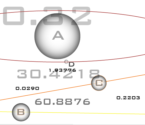
slider row 1: 60.8876, 1.9285, 196.440, 0.0290, 139.356

slider row 2: 30.4218, 0.6174, 358.317, 0.2202, 156.648

slider row 3: 1.9378, 0.0185, 218.012, 0.0000, 0.0000

velocity offset #1: 13.94 m/s

velocity offset #2: -45.16 m/s