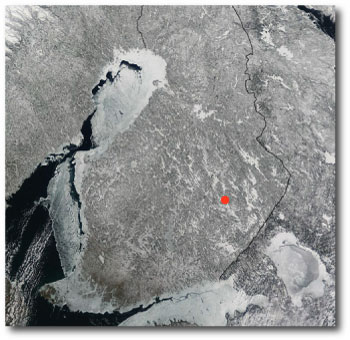
Varkaus

Varkaus

Image source: NASA Visible Earth

For most people, a mention of Finland brings to mind snow, lakes, conifers, Nokia and Linus Torvalds. Here at oklo.org, however, we hear Finland and we think of top-drawer amateur astronomers. In 2000, the Finn Arto Oksanen was the first amateur to observe the HD 209458 b transit. More recently, both Oksanen and countryman Pertti Paakkonen have contributed a number of observations of TrES-1 and other stars to transitsearch.org. Finnish IP addresses are consistently among the top traffic generators on the Systemic Console.

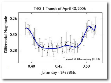
Now, Veli-Pekka Hentunen and the Warkauden Kassiopeia ry (the Astronomical Association of Varkaus) join the ranks, with a fine observation of last week’s TrES-1 planetary transit. Their lightcurve, shown just below, was obtained with a Meade 12-inch LX200 telescope and a cooled SBIG ST8-XME CCD camera:

April 30, 2006 TrES-1 Transit Photometry

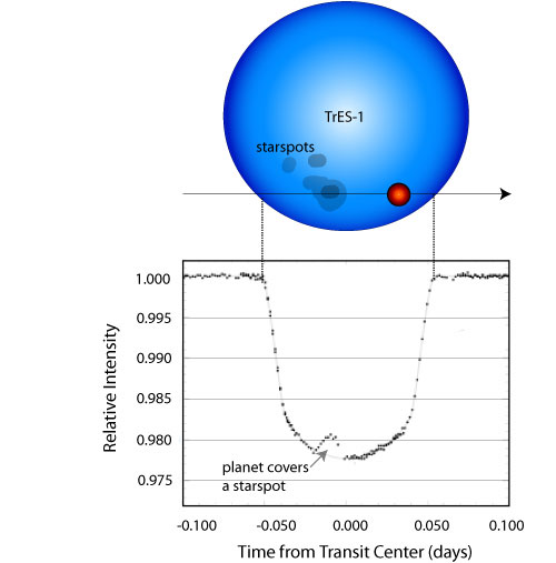
The photometry shows a tantalizing hint of the starspot activity that is known to characterize TrES-1. A more detailed analysis will be needed to see whether the small in-transit bump has statistical significance. As discussed in a previous post, HST has shown that starspot activity on TrES-1 can produce stange-looking features in the light curve:

transit of TrES-1 obtained with HST

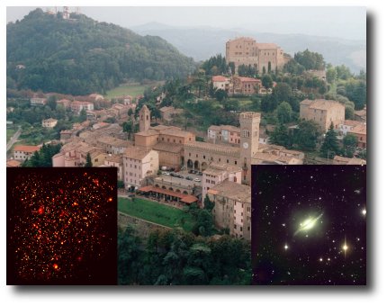
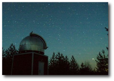
Hentunen and his colleagues have constructed a very impressive facility at a dark (and from the look of things cold) site in the Finnish interior. Information in English regarding both their observatory and their scientific work can be found at the Taurus Hill Observatory Website.

varkaus observatory

Taurus Hill Observatory

Hentunen and friends will be able to kick back and take it easy for the next few months because it doesn’t really get dark at their location during the Summer. In the Winter, however, when the weather is clear, they’ll have the opportunity to make long-duration time-series photometric observations of stars near the polar cap. For example, they’ll be in awesome position to snag oklo.org favorite HD 80606 (+50 deg declination) during its Dec. 26, 2006 transit opportunity.

tilt shift

When it comes to planetary systems, our own eclectic gathering of eight (or nine, or ten) planets is by far and away the best characterized and best understood. We’ve flung space probes past all of the planets in the solar system, and we’ve directly, physically, probed four of them (in addition to two major satellites). We know their orbits to stunning, uncanny precision. We have actual pieces of Vesta and Mars under minute scrutiny in our laboratories. We have coffee table books overflowing with detailed photographs our our home worlds.

a detailed view of a surface feature on a life-bearing habitable planet

I can step right outside my door and photograph the surface details of a habitable terrestrial planet.

Sadly, we don’t have anything rembling this wealth of detail when it comes to extrasolar planets. Most of our information is encapsulated in the tables of radial velocity measurements accessible to the Systemic Console. Much of what I write about in these posts, and indeed, most of what we can infer about these distant worlds, must be squeezed from sparse columns of times, velocities, and velocity uncertainty estimates.

(more…)

Where we’re at

banana leaf

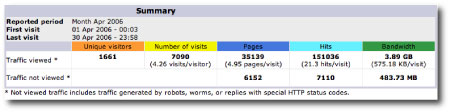
The systemic collaboration website has now been on the air for six months. Traffic has been increasingly steadily. By the end of April, oklo.org has been averaging 250 visitors a day, with a total of 1661 unique “real” visitors for the month. (This brings to mind a philosophical question: if a tree falls in a forest, and only robots, worms, or replies with special HTTP status codes comment, did it make a sound?)

april showers

The Systemic Team is enthusiastic about a number of improvements that will be coming on line very soon. Here’s a rundown of what to look for during May:

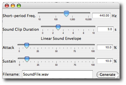
1. Aaron Wolf is putting the finishing touches on the next release of the systemic console. The updated version will have a number of subtle improvements to the existing controls, and will have several completely new features, including a sonification utility and a folding window. Sonification allows the user to create a .wav format audio file of the radial velocity waveform produced by a given configuration of planets orbiting a star:

console sonification controller

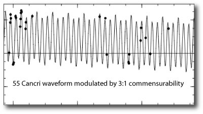
As we’ll discuss in future posts, the ability to “listen” to dynamical systems provides a startlingly effective and completely novel way to evaluate the long-term orbital stability of a hypothesized system of planets. For example, when a configuration of planets is stable, one generally gets a sound with a steady timbre: [example 1.5 MB .wav file corresponding to a stable planetary system].

On the other hand, when a configuration of planets is unstable, the radial velocity waveform of the star can get pretty crazy, which can lead to an inifinite variety of very weird sounds: [example 0.5 MB .wav file corresponding to a dynamically unstable planetary system].

2. Stefano Meschiari, who will be transferring as a graduate student to the UCSC graduate program this Fall (yes!), has developed a PHP-based collaborative environment for the systemic project. Think flickr, think myspace, think the Extrasolar Planets Encyclopedia, think seti@home, and think effective scientific collaboration all rolled into one. I’m not kidding, folks, it’s amazing.

G.I. No

planet formation is not yet in focus

In a comment on yesterday’s core-accretion post, a reader anticipated that all is not hunky-dory with the core-accretion scenario for the formation of the gas giant planets in our solar system, and asked if is there any support for Alan Boss’ disk instability model. In the Boss model (described here by Alan, see also the buff 137-strong citation list) gas giant planets condense directly out of the protostellar disk as the result of gravitational instability in the disk.

The handy thing about an extrasolar planet web log is that you can express your opinions on the formation of extrasolar planets. In my opinion, there are a number of very serious difficulties with the hypothesis that gravitational instability is the dominant mechanism for giant planet formation. Here are three:

(1) In order to have gravitational instability work in the manner shown in the fragmentation simulations, you need to start with an axisymmetric disk that has a sufficiently low value for the Toomre Q parameter. That is, in order for the initial conditions in the successful Boss simulations to be valid, a growing protostellar disk needs to remain completely stable with respect to low-level non-axisymmetric disturbances until BOOM, it reaches a threshold Q value where it is prone to spiral instabilities that exponentiate on a near-orbital timescale.

In reality, I think that a growing (or alternately, a cooling) protostellar disk will be prone to low-level spiral disturbances that steadily transport mass inward and angular momentum outward, allowing the disk to avoid ever reaching the state where instabitilies can grow on an orbital timescale. (For a bulked-up version of this argument, see the papers (one and two) that I wrote with Vladimir Korchagin and Fred Adams on this issue).

(2) The core accretion model provides a very natural explanation for both the planet-metallicity correlation, as well as the paucity of Jovian-mass planets found in orbit around low-mass M type stars. The gravitational instability model predicts that the incidence of Jovian-mass planets should be independant of both the stellar metallicity and the parent star mass.

(3) There’s simply no way that the gravitational instability model can produce the 72 Earth Masses of heavy elements in HD 149026 b. (See this paper for a thorough discussion).

To be fair, there are also some thorny problems associated with core-accretion. In the next few posts of the giant planet formation series [1, 2, 3, 4 and 5] that we’ve been running, I’ll describe these in more detail.

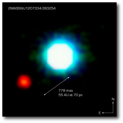
Planet Orbiting a Brown Dwarf

Photo credit: ESO (VLT/NACO)

Another important point to stress is that Alan’s simulations certainly aren’t in error in the sense of being computationally wrong. It’s just that I don’t agree with the generic validity of the initial conditions. Indeed, I do think that gravitational instability sometimes plays a role in giant planet formation. The best example is probably the 5 Jupiter-mass companion to the brown dwarf 2M1207 discovered by Chauvin et al. last year. (The ESO press release on this system is here.) I see no way in which the core-accretion process could have made any headway at 55 AU in this particular system.

Finally, GJ 876, which is by far the best RV-characterized extrasolar planetary system, provides a tough challenge to both the gravitational instability and the core-accretion theories. The inner 7.5 Earth Mass planet in the GJ 876 system is almost certainly an accreted protoplanetary core (regardless of whether it formed in-situ, or migrated from a larger radius). It would be nearly impossible to form lil’ D via gravitational instability. The outer two planets, on the other hand, contain more than three Jupiters worth of mass, and stand in embarrassing conflict with the notion that core-accretion process is difficult to carry through to Jovian-mass completion in red-dwarf protostellar disks.

I would very much like the 411 on what went down in GJ 876’s protostellar disk.

Oligarchic Growth

[A continuation of posts 1, 2, 3, 4 and 5 on the formation of Jovian planets.]

nucleus of a comet

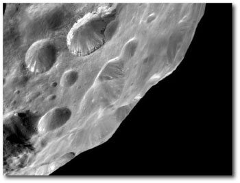
Phoebe (photographed by Cassini). The cores of the giant planets were built from millions of these objects.

In the primitive solar system, ice formed at the expense of water vapor wherever the temperature was lower than 150 degrees above absolute zero. The 150 K isotherm in the disk was located roughly at Jupiter’s current distance from the Sun, and is known colloquially as the “snowline”. Just beyond the snowline, the planetesimals achieved their greatest ability to rapidly build themselves into larger bodies. It was cold enough for ice to be stable, yet close enough for the overall density of the disk to be high, and the planetesimals were prone to frequent collisions.

Low-speed planetesimals collisions were sticky events that can be simulated to wonderful effect with fast desktop computers. Imagine two Michelin Men, each loosely glued together, heading toward each other in a headlong embrace. A spare tire or two is lost in the collision, but one remains with a jumbled, combined mess. The first planetesimal collisions that seeded Jupiter’s core looked something like that.

Thousands of years passed, punctuated by these (initially) slow-motion catastrophes. The planetesimals gradually become fewer in number and individually larger. Those that experienced a few extra collisions in the beginning were able to take advantage of their burgeoning self-gravity to collide more often, and were thus able to grow faster (sound familiar?) Inevitably, a few big winners, called oligarchs, began to emerge. These oligarchs, with radii thousands of miles across, were massive enough to simply haul in their neighboring small-fry kilometer-sized brethren. The more an oligarch gets, the more it wants, and the farther its reach. A runaway occurs. Somewhere in the current vicinity of Jupiter, 4.54 billion years ago, an oligarch reached an Earth mass.

three stages of core accretion

What would this oligarch have been like? Certainly, it would be something that we would have little difficulty calling a planet in distress. All riled up. A five hundred mile wide core of molten iron, surrounded by perhaps a thousand miles of pressurized plastic rock, not unlike the mantle of the Earth. Above that, thousands upon thousands of miles of hot, pressurized, water ocean. Floating atop the ocean, a tarry layer of hydrocarbons, perhaps with a smell like hot asphalt, and with an indistinct surface merging into a choking thick noxious atmosphere.

The atmosphere bulks up fast. Liberated hydrogen and helium gas bubbles up from the layers of denser materials in the interior. The oligarch passes several Earth masses in size, and grows massive enough to grab gas directly from the disk. Meanwhile, new planetesimals are arriving all the time. Kilometer-sized projectiles streak through the exosphere, exploding as they slam into the atmosphere. The unsettled skies are continuously ablaze with meteors. The temperature rises, becoming so warm that the atmosphere glows a dull coal-red in the darkness of the nebula.

When the growing oligarch, now a full-fledged protoplanet, reaches seven or ten times the mass of the Earth, it is pulling in gas as fast as it can. The atmosphere has swelled and bloated to a thickness of literally hundreds of thousands of kilometers. The gas glows fire-engine orange, and pours infrared light out into space. This radiation is accompanied by slow settling of the lower layers, providing room at the top for more gas to flow in.

Finally, the growth experiences its first taste of a slowdown. The consumption of rocky icy planetesimals has been so rapid that the total reservoir of these objects in the annular region of the nebula occupied by the planet is depleted. The planet has managed to effectively clear out the solid material from a vast ring-like region of the nebula. The region around the protoplanet still contains vast quantities of gas, but this gas is prevented from accreting onto the bloated planet. The planet can only add new gas as fast as the older gas is able to settle, and the gas can only settle by radiating and cooling.

For the next million years, the planet grows slowly. Gas flows in from the disk as fast as the cooling of the planet will allow, and as the mass of the planet increases, the annular ring of the disk from which planetesimals can be drawn also slowly increases in size…

Dexter

glasses

Some of the planets that have been detected via the radial velocity technique have been announced in the refereed literature without the supporting evidence of a published table of radial velocities. For the planets that fall in this category, the end-user gets a star name, a list of orbital elements for the planet, and a graph showing a model velocity curve running through the data points. Occasionally, the data is folded, and only a .gif file of the phased radial velocity fit is published.

In a previous post, I wrote about why I can certainly appreciate the planet detection teams’ reasons for not wanting to divulge their radial velocity data when they announce a new planet. If a star has one detectable planet, then the odds are about 50-50 that another planet will be detected after several additional years of monitoring. For a variety of reasons, multiple-planet systems are scientifically more valuable than single-planet systems. In particular, a multiple-planet system (such as GJ 876) tells a fascinating dynamical story, which in turn yields valuable information about the formation and evolution of the planetary system. Obtaining radial velocities is hard, expensive work.

The unavailability of the radial velocity data sets for some of the planet-bearing stars has led to something of a gray market industry in which the radial velocity plots of the parent stars of interesting multiple-planet systems such as HD 82943 and HD 202206 are digitized, and the radial velocities are reconstructed from the graphs. For an example of this technique, see this preprint on astro-ph.

I bear some of the responsibility for the radial velocity .gif digitization industry. In 2001, a press release was sent out announcing the discovery of eleven new planets. This bumper crop included two particularly amazing systems, HD 80606, and HD 82943. HD 80606 harbors a massive planet on an extremely eccentric orbit, and I was very interested to fit the data myself in order to estimate the uncertainties in the transit windows.

The tabulated radial velocities on which the fits were based were not published, but postscript files showing plots of the radial velocities versus time were posted. I went into the files, and by placing commands to print characters in red, I was able to figure out how the plot was encoded. I was then able to extract the exact measured radial velocities for both HD 80606, and HD 82943 from the press conference postings. I didn’t try to publish the analysis that I did with this data, since the procedure seemed a little under-the-table. I did tell people what I was doing, however, and the radial velocity plots on the websites were soon changed from postscripts to .gif files, which are much harder to reverse-engineer.

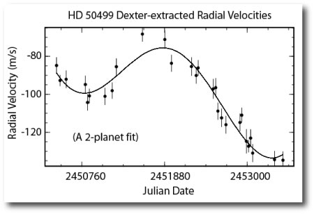
One of our initial goals with the systemic collaboration is to provide the ability for anyone who is interested to perform a uniform analysis on all of the radial velocities underlying all of the published planets that make up the current galactic planetary census. In order to do this, we need a mechanism for accurately extracting the data from image files in .gif and .jpg format. Systemic team member Eugenio Rivera has been working on this, and has been getting good results with the Dexter Java Applet (available from ADS). The ADS information page gives the following overview:

Dexter is a tool to extract data from figures on scanned pages from our article service. In order to use it, you need a browser that can execute Java Applets and has that feature enabled. Netscape users can verify this by selecting “Edit” -> “Preferences” -> “Advanced” from the top-bar menu and making sure that the button “Enable Java” is checked.

Dexter can be quite useful in generating data points from published figures containing images, plots, graphs, and histograms, whenever the original datasets used by the authors to produce figures in the papers are not available electronically.

We’ll be posting velocity sets extracted from .gif files shortly, and Eugenio will post a detailed write-up of the technique and pitfalls of “observing” the observations.

Mötley Crüe

Mt. Hamilton at Dusk

Mt. Hamilton Main Building at dusk, photo by Laurie Hatch

Last weekend, I wrote a post about the planet — stellar metallicity connection, and the small-scale Doppler-velocity planet search that Debra Fischer and I carried out at Lick Observatory as a precursor to the currently ongoing N2K survey.

We had eighteen candidate stars on our list, ordered in terms of increasing uvby-determined metallicity, and to keep track of them, we named them after heavy metal bands:

table of heavy metal bands

We started observations in September 2000. Several times a month, I would drive up the twisting road to Mt. Hamilton, windows open to the dry chaparral air. At the mountaintop, the observatory buildings on the ridgeline sleep in the hot quiet afternoon sunlight. The scene seems lost in a slower, less hectic time. E-mail, phone messages, deadlines, all-hands division meetings are far away and inconsequential.

After standing and staring for a long time at the sweeping expanse of ridges, mountains and valleys spreading out in all directions, I would pick up a set of keys, a flashlight, a thermous of coffee, and a night lunch from the diner, and walk to the dome.

Once inside, the lost-in-time feeling immediately gives way to the scramble to set up for the night. Open the spectrograph, fill the ccd dewar, focus the optics, set up the iodine cell, obtain the thorium-argon calibration and flat-field images, check the telescope pointing, and run through a number of other ordered tasks, all of which are required for a successful night of observations. We were using the then-undersubscribed 1-meter Coude Auxilliary Telescope, which has a certain Rube-Goldberg aspect to its inner workings. It took all (and more) of my clumsy theorist’s mechanical aptitude to make sure that I didn’t skip a step of the complicated set-up procedure.

Eventually, with the sky grading into deep blue twilight and the night’s first target star acquired, the stress associated with the set-up procedure would dissipate. Because of the small size of the telescope, the individual exposures were long and unhurried. I’d take two and sometimes even three separate half-hour exposures. With the shutter open, with starlight streaming through the iodine cell, reflecting off the spectrograph, and landing on the CCD, there was little to do aside from making sure that the autoguider was doing it’s job of keeping the star centered on the spectrograph entrance slit.

After three months, several of the stars were showing tantalizing hints of short-term radial velocity variablility. All of our main-sequence target stars have “F-type” spectra, meaning that they were somewhat more massive (and thus hotter) than the Sun. It was impossible to get the 3-5 m/s precision that can be obtained with slightly cooler solar-type “G” stars. For F-type stars, the metal lines that greatly aid the measurement of precise Doppler shifts are starting to fade, and, because F-type stars are generally quite young, they are often rapidly rotating. Unless the star is being viewed pole-on (which seems to be bad for planet detectibility) stellar rotation broadens the spectral lines and further degrades the velocity precision.

Mötley Crüe, in particular, was exhibiting radial velocity variations that seemed to strongly imply the presence of a short-period planet. This was mildly surprising, given its rather puny, barely super-solar “80’s hair metal” metallicity of [Fe/H] ~ 0.04 dex. We became more and more excited, as each velocity seemed to come in on target:

Early Radial Velocitis for Motley Crue

I have to go and teach a class now, so I’ll pick up the story sometime during the next few days. Also, when I get back from class, I’ll add the velocities shown in the figure above to the Systemic Console under the name “Mötley Crüe”. If you’re interested, you can then do a quick analysis which will show you why Debra and I were getting excited by the velocities.

Agglomeration

[A continuation of posts 1, 2, 3, and 4 on the formation of Jovian planets.]

dust bunny on a flatbed scanner

The idea that the planets in our solar system arose from a flattened, rotating cloud of gas and dust dates back to Kant and Laplace in the 1700s. Their so-called nebular hypothesis drew part of its original support from the spurious suggestion (by William Herschel and others) that the spiral “nebulae” such as M31 in Andromedae might be solar systems caught in the early phases of formation.

By the late 1800s, however, it had become clear that spiral galaxies are most certainly not protoplanetary disks. This realization removed a primary pillar of observational support for the nebular hypothesis, and forced theories of planet formation to rest largely on assumptions and theoretical arguments. For the majority of the twentieth century, astronomers trying to figure out how the planets came to be were forced to work backward from the more or less static clues that are provided by the condition of the solar system today. Not a happy situation. Science works best with direct observations. To really understand how planets form, we really need to see the formation process in action.

As it turned out, protostellar disks around newborn stars were observed before the discovery of the first extrasolar planets. In the early 1980’s, the IRAS infrared satellite discovered that Beta Pictoris, a young, apparently ordinary, sun-like star 53 light years from Earth, was glowing unexpectedly brightly in infrared light. When Beta Pictoris was examined with careful follow-up observations, it was found to be orbited by a large flattened disk of dusty particles. After this first discovery, many more protoplanetary disks were discovered. Beautiful examples occur, for example, in the Orion Nebula, where they are imaged by the Hubble Space Telescope in stark rigid detail against a glowing backdrop of nebulosity. From careful study of these disks, we know that they generally contain anywhere from 1 to 100 times the mass of Jupiter, and are composed primarily of hydrogen and helium gas, along with swarms of dust and icy particles.

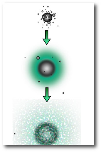
If we assume that giant planets do not condense directly out of these disks as the result of gravitational instability, then we need a coherent picture for forming the planets that we know actually do exist. The current best-guess scenario for forming Jovian-mass planets is called the core accretion theory.

In the core accretion picture, planets start small, through the buildup of dust.

If you have a hardwood floor, you can develop a hands-on sense of how dust agglomeration works by refraining from vacuuming under the bed. If you do this, you will notice that the dust does not accumulate in a uniformly thick layer with time. Rather, the presence of slight air currents swirls the dust around, and causes it to build up into dust bunnies. Look at a dust bunny under a magnifying glass, or put it on a flat-bed scanner and import it into photoshop (that is what I did to generate the image at the top of this post). It’s mostly air. The dust – hair, dandruff, unidentifiable strands of ticky-tacky, has a structure that takes up a large volume in comparison to its mass. This property makes it effective at scooping up more material. Once dust agglomerations begin to grow, their subsequent growth becomes easier. A similar agglomerative process may be at work in building up the dust agglomerations that are present in protostellar disks.

Even so, the initial growth of dusty, icy objects in a proto-planetary disk seems fraught with difficulty. The problem is that as the dust-ice agglomerates become larger and larger, they experience a headwind from the gas in the disk. This headwind causes them to spiral inward, eventually vaporizing as they get close to the central star. Some mechanism must exist to concentrate the dusty debris and allow it to build in size more quickly than it can be destroyed through spiraling inward. There seem to be two reasonable candidates for sequestering dust. The protoplanetary nebula might contain vortices, that is, storm systems in the disk itself, in which regions of the disk participate in a hurricane-like flow pattern. Numerical simulations show that disk vortices, if they live long enough, can trap and concentrate solid particles in their centers. Another possibility is gravitational instability (of a more restricted type than dramatic variety described in post #3). If the gas in the disk is flowing very smoothly, then the solid particles in the flow will have a tendency to settle to a thin layer at the disk mid-plane. If this mid-plane layer grows dense enough and massive enough, then a gravitational runaway can occur. The solid particles, the dust, the ice, the gravel can rapidly form larger and larger objects. Once these objects attain a certain size, several tens of kilometers, say, they are safe from the drag force exerted by the nebular gas. A best-guess scenario has tens of trillions of kilometer-size planetesimals emerging in the disk a hundred thousand years or so after the disk forms.

three initial phases of giant planet formation
Trillions of planetesimals sounds like a lot. Nevertheless, the disk at that stage would not have seemed particularly crowded. The density of gas would have been thousands of times less than the density of air, and the distance between kilometer-sized bodies would be measured in thousands of miles. If you could transport yourself to a random point in the middle reaches of the disk, there would seem to be only relentlessly empty blackness. No view of the stars, no view of the young forming sun. It would seem as if nothing had changed from the earlier molecular cloud phase.

A thermometer, however would indicate that a difference does exist. Whereas the molecular cloud was incredibly cold, 5 or 10 degrees above absolute zero, the temperatures in the protostellar disk are much warmer, ranging from hundreds, even thousands of degrees very near the star, down to several tens of degrees above absolute zero in the farthest reaches of the disk.

Roboscope

DSS2 Red Image of GL581

Last week, we posted Kent Richardson’s light-curve for the nearby red dwarf star GL 581 (Sloan DSS image pictured above). Kent’s photometry was taken during a predicted transit window, and along with data from David Blank and collaborators in Australia, it contributed to rule out the possibility of planetary transits by the red dwarf’s steamy Neptune-mass companion.

Like Marlon Brando in On the Waterfront, GL 581 b “could’ve been a contender”, and connoisseurs of the might-have-been should be sure to read the oklo posts [1,2] that talk about what this planet would have taught us if only it was transiting…

No need to despair, however. There’s a whole slew of candidates on the transitsearch.org candidates list which remain entirely unexplored.

Kent obtained his data with a robotic telescope located at the San Diego Astronomy Association’s dark site at Tierra Del Sol, California, approximately 60 miles east of downtown San Diego:

sdaa roboscope

Kent reports,

There are three major components of the installation: The dome and telescope, the data cabinet, and the satellite antenna. The details of each are as follows:

Dome
Robo Dome by Technical Inovations, Inc.
Meade 8″ LX-200 Classic f/10
Meade f3.3 Focal reducer
SBIG ST-7 CCD camera w/ CFW-8 filter wheel
Lumicon 80mm finder scope w/ Meade DSI Pro camera
Meade 8x50mm finder scope with Logitec web cam

Data cabinet
Compaq Presidio desktop computer
The Sky for telescope control
CCDSoft for ST-7 control
Meade Autostar Suite for DSI control
Logitec Image Studio for web cam control
Digital Dome Works for dome control
Tachyon Networks Inc. satellite network computer

Satellite Antenna
Tachyon Networks Inc. satellite dish

The photo shows the site. The data cabinet has been wrapped to protect it from the winter rains we have been experiencing. You can also see a second pier and electrical outlet which will enable us to install another dome and telescope when funding is available.

We’re definitely looking forward to seeing more data from this rig when the California weather finally improves.

In other news, Transitsearch.org and the American Association of Variable Star Observers have just announced a joint campaign to search for transits of the recently discovered planet orbiting HD 33283. There’s one last, fleeting window of opportunity this season before the star goes behind the Sun: April 26, 10:31 – April 27, 20:22 (UT). Details of the campaign can be found here.

Seize the moment!

Metal

aluminum foil on a flatbed scanner


51 Peg
is an ordinary star in nearly every respect. It is, however, more metal-rich than the Sun by nearly a factor of two, which gives it a metallicity in excess of all but a few percent of the stars in the local galactic neighborhood.

When Astronomers talk about metallicity, they mean the fraction of a star’s mass that is contained in elements that are heavier than hydrogen and helium. To an astronomer, carbon, nitrogen, krypton, and radon are all “metals”. In the Sun, metals comprise a bit less than 2% of the total mass.

Nearly every parent star in the first wave of extrasolar planets (including 55 Cnc, Tau Boo, and Ups And) came in with considerably higher-than-average metallicity, and the strong connection between high stellar metallicity and the detectable presence of an extrasolar planet was on fairly secure footing by 1997. This connection has been quantified very clearly, and is perhaps the most important and dramatic result that come out of the first decade of investigation of extrasolar planets. The figure from Debra Fischer and Jeff Valenti’s recent paper is fast on its way to iconic status:

the planet metallicity correlation

The planet-metallicity connection is telling us something important about the planet formation process, namely, that the core-accretion mechanism for forming giant planets is correct. (More on this coming up soon.) It also tells us how to efficiently find more planets. If you want to find planets, look at metal-rich stars.

Purists should definitely argue that by skimming the readily detectable planets from metal-rich stars, one is skewing the statistical properties of overall census of planets, while introducing additional systematic trends into a planetary catalog that is already shot through with biases both subtle and overt. “A targeted quick-look Doppler survey of metal-rich stars is the moral equivalent of eating candy for breakfast!”

I fully agree.

There are, however, scientifically compelling and unassailably selfless arguments for why it’s important to locate as many extrasolar planets as quickly as possible. I think the most important reason is that quick-look radial velocity surveys (such as N2K) are the best way to locate planets that transit bright parent stars. Once identified, objects like HD 149026b yield up a simply incredible amount of information.

But I’ll be straight with everyone. I’ve always wanted to be in on the discovery of new planets.

In 2000, I worked with Debra Fischer on a small-scale survey of metal-rich stars that wound up being the precursor project to N2K. It’s hard to imagine that the year 2000 once seemed like the distant future. At that time, it appeared that in addition to the planet-metallicity correlation, that there was also a planet-stellar mass correlation. The census of short-period planets known in 2000 was noticeably concentrated around stars somewhat more massive than the Sun, that is, early G and late F type stars.

I therefore drew up a list of 20 stars that we could observe using the then-undersubscribed CAT (Coude Auxilliary Telescope) on Mt. Hamilton. The criteria for inclusion were that a candidate star be (1) at least moderately metal-rich, (2) bright, (3) more massive than the Sun, and (4) not known to be on any other radial velocity survey lists. We needed stars brighter than about magnitude 6 because the CAT telescope has a mirror diameter of only one meter.

Rapidly, it became clear that Henry Draper catalog numbers are not a very effective way to mentally keep track of the stars. There was confusion, for example, one night when I asked Debra if I could add “HD Twenty –Six Seven Five” to the evening’s observing list. She thought that I meant “HD 2675 “(which had already set), when I actually had “HD 20675” in mind. We eventually realized that since we needed to keep both the stars and their metallicities straight, the best course of action would be to name the stars after heavy metal bands. At the high-metallicity end, we drew on speed-metal and death-metal outfits (e.g. Slayer, Sepultura), wheras at the lower-metallicity end, we resorted to hair-metal and even glam-metal bands (i.e. Warrant, Skid Row). Here’s our final list of stars in the survey:

table of heavy metal bands

(The original twenty star survey was reduced to eighteen after AC-DC turned out to be a spectroscopic binary, and W.A.S.P. turned out to be chromospherically active.)

rates

In astronomically inclined households, the first wave of extrasolar planets to be discovered, 51 Peg, 70 Vir, Ups And, Tau Boo, are all still household names.

cactus pad

With the later additions to the census, however, such as HD 33283 b et al., even the discoverers can have a hard time keeping the names in mind. In part, this is because it’s tough to keep a bunch of random Henry Draper Catalog numbers at the tip of the tongue. It’s also because planets #184, #185, and #186 don’t quite pack the same panache as planets #2, #3, and #4. Maybe it’s time to start naming these planets?

It’s easy to get the impression that the rate of discovery of extrasolar planets is increasing rapidly with time. Interestingly, however, this hasn’t been the case recently. The planet discovery rate peaked in 2002, with 34 planets detected, and the rate over the last four years has been flat, at about 25 planets per year. (The present year has brought us six new worlds during the span between New Years Day and Earth Day):

rate of planet detection

The detection rate has flattened for several reasons. After a decade’s worth of planet discoveries, the Doppler radial velocity method remains the most productive technique. The radial velocity method is most efficient when one has a bright parent star. Most of the suitable stars with V magnitudes brighter than 8 are already on the Doppler Surveys. The readily detectable short-period planets orbiting these stars have mostly been found. The much longer orbital periods of the outer planets mean that one must be increasingly patient as one waits for new discoveries from venerable stars. Indeed, the detection rate of planets over the past several years would be even lower, were it not for targeted Doppler surveys such as N2K, which are specifically designed to find new planets quickly by surveying metal-rich stars.

The transit and microlensing methods have a lot of promise for upping the planet detection rate, but to date, very few planets have been discovered with these techniques. In an upcoming post, we’ll look in more detail at the reasons why this has been the case.

It’s interesting to compare the planet detection rate with the history of minor planet detections. Ceres, the first minor planet to be discovered, was found in 1801, followed by Pallas in 1802, Juno in 1804, and Vesta in 1807. A thirty-eight year gap followed, until the discovery of Astraea in 1845. The 100th asteroid, Hecate, was found in Ann Arbor Michigan in 1868, and asteroid #188 (equal to the number of extrasolar planets currently known) Minippe was found ten years later in 1878. The rate has increased rapidly since then. As of last November, there were 120,437 numbered asteroids:

discovery rate for asteroids

I think it will take about 15 more years to find 120,437 planets.

2010

correlations?

As I’ve mentioned earlier, Jean Schneider’s authoritative Extrasolar Planets Encyclopedia has introduced a slick .php-based approach that’s keeping the systemic team on their toes. At Schneider’s site, one can interactively produce correlation diagrams for the known extrasolar planets. As more planets are discovered, these diagrams (for example the a-e plot and the Msin(i)-a plot) are beginning to show a fascinating richness of detail.

The inclusion of date of discovery as one of the plottable parameters attracted my attention.

For example, a plot of the Log of the planetary period versus discovery date shows hints of interesting structure:

planetary period vs. discovery date

Over the past few years, the majority of newly detected planets can be divided into a population with P<10 days (the hot Jupiters), and a population with P>200 days (the eccentric giants). There is a statistically significant gap in the period distribution in the intermediate-period regime. This gap tells us something significant about the planet formation process. My interpretation is that the migration process is not readily halted until a planet reaches the region of the disk where the dyanamics of the protostellar disk gas are subject to the laws of ideal MHD. More on that later.

From a more practical standpoint, the paucity of intermediate period planets has made it tough going for the transitsearch.org collaboration. When planetary periods are less than about 10 days, the discovery team is usually able to complete a photometric search for transits before the planet is publicly announced. When a planetary period exceeds 200 days, it’s generally hopeless to mount an exhaustive transit search, even with a distributed network.

You’ll get another very interesting diagram if you plot the Log of the planetary mass as a function of discovery date. As usual, I’ve redone the axes and annotations with Adobe Illustrator to get that familiar oklo.org look-n-feel:

planetary mass vs. discovery date

In this log-linear space, the lower envelope of detected planet mass is a linear function of time. This allows for an easy extrapolation to estimate the discovery date of the first Earth-mass planet orbiting a nearby main-sequence star…

Three new planets

Yesterday, John Johnson and the California-Carnegie Planet Search Team posted an astro-ph preprint announcing the discovery of three new extrasolar planets. All three radial velocity data sets have been added to the Systemic Console, and the transit predictions have been placed on the transitsearch.org candidates list.

HD 86081 b has an orbital period of 2.1375 days, which makes it a long-sought “missing link” between the weird, ultra-short period planets discovered by the OGLE survey and familiar hot Jupiters such as HD 209458 b and 51 Peg. HD 86081 b has been checked photometrically for transits, but unfortunately, they don’t occur. Because HD 86081 b orbits so close to its parent star, the a-priori transit probability was a healthy 17%.

HD 224693 b and HD 33283 b have longer periods of 26.73d and 18.179d, respectively. The parent stars are excellent targets for the transitsearch.org project, as neither one has been monitored photometrically during the centers of the transit windows. The a-priori transit probability for HD 33283 b is an impressive 6.2%, whereas HD 224693 tosses in a 3.2% chance. That’s a 9.4% chance that a small-telescope observer will be a world-famous astronomical hero sometime during the next year…

Dust off those CCD cameras!

GL 581. Flat, unfortunately.

wheat

Regular visitors to oklo.org are familiar with GL 581 b, a Neptune-mass planet in a 5.366 day orbit around a nearby M-dwarf star. I’ve developed a fascination with this planet, because if it can be observed in transit across the disk of its parent star, then we will learn an incredible amount about the planet’s interior structure. In a nutshell, if the planet has a small transit depth then we’ll know it’s made of rock and metal, and if it has a larger transit depth, then we’ll know it’s made mostly of water.

The a-priori geometric probability that transits by GL 581 b occur is 3.6%. Because the planetary orbit is fairly well known, the time windows during which transits can occur are fairly narrow. The expected transit depth for the planet (if it’s made of water) is a respectable 1.6%, which means that observers with small telescopes will be able to detect the transits if they are occurring.

For more details on the GL 581 campaign, please read (1) this oklo post, “clouds”, and then (2) this oklo post, “two for the show”. For information on how amateur astronomers and small-telescope observers can participate in the search for transiting extrasolar planets, see our website for transitsearch.org. Over the coming months, we’ll be integrating transitsearch.org much more tightly into the oklo site. The systemic project and the transitsearch project both have a common goal of facilitating meaningful public participation in cutting-edge extrasolar planet research.

Every 5.366 days, I’ve been peppering the transitsearch.org observers mailing list with exhortations to observe GL 581 during the transit windows. The weather has not been very cooperative, and many opportunities worldwide were thwarted by clouds, but we now have two data sets that indicate that transits by GL 581 b are unlikely to be occurring:

gl581 photometry

The top data set (from April 2nd) was obtained by David Blank and Graeme White (of James Cook University) using a robotic Celestron C14 stationed at the Perth Observatory. The observations were made through an uncalibrated R filter. The operation of the telescope is made possible by the Perth Observatory staff Jamie Biggs and Arie Verveer, with Carl Pennypacker participating remotely from UC Berkeley. The bottom data set, from April 12th, was obtained by Kent Richardson, using the transitsearch.org robotic telescope, which was set up by Tim Castellano, and which is located in San Diego.

Sadly, neither data set shows any hint of a transit. In addition, David Blank has another data set in hand from March 28th, which also shows no sign of transit. I’ll update the post shortly to include that set as well. Several more observations will be required to really scratch GL 581 b off the list, but at this point it doesn’t look good for transits.

So yeah, I’m a little bummed out. But look at the bright side. A worldwide network of small-telescope observers has obtained an important astronomical result, demonstrating the feasibility of the transitsearch.org approach. If we keep observing the candidates, eventually we’ll hit pay dirt.

Q

This post continues the oklo.org posts: (1) the black cloud, and (2) disks.

spiral waves in m51

There are two competing, completely distinct theories that describe how a giant planet like Jupiter can be generated from a protostellar disk of gas and dust. The first theory, formation via gravitational instability, lends itself to large-scale hydrodynamical simulations and extraordinary animations that can be downloaded over the Internet. It’s an easy theory to grasp. The second theory, formation via core accretion, presents a more complicated chain of events, but nevertheless contains the story that seems (in my opinionated opinion) to be most nearly correct. Let’s look at what these two theories say, and let’s examine the evidence in favor of and against each.

In the gravitational instability picture, the outer lagging remnants of the molecular cloud core fall in and land on the protostellar disk, causing it to grow in mass. As the disk mass increases, it begins to be influenced by its own gravity. That is, it starts to feel a tendency to fragment in response to its own weight. Simultaneously, the pressure of the gas in each nascent fragment pushes back and partially offsets the fragment’s inclination toward collapse. Pressure thus acts as a small-scale stabilizing influence against collapse. In addition, the differential rotation of the disk (material closer to the star orbits faster) tries to sheer a growing fragment apart. Differential rotation thus acts as a large-scale stabilizing influence against gravitational collapse.

The question boils down to the following: Does gravity win, allowing a Jupiter-mass planet to rapidly form as a condensation in the disk, or do shear and pressure win, keeping the disk free of giant-planet fragments?

The situation lies within the general framework of a linearized hydrodynamical stability analyses, and can be analyzed mathematically. The analysis leads to a so-called stability criterion, the famous Toomre Q:

toomre q

Where c_s is the sound speed in the disk, kappa is the epicyclic frequency, G is Newton’s gravitational constant, and sigma is the disk surface density. If Q<1 at any radius in the disk, then the disk is unstable with respect to m=0 (ringlike) disturbances. If Q is slightly greater than 1, computer simulations show that the disk is prone to strong non-axisymmetric instabilities, and hence experiences exponential growth of disturbances and eventual fragmentation.

As with any seemingly abstruse physical phenomenon, The disk instability analysis can be illuminated with an analogy. In this case, the appropriate analogy involves a rock band, a house party, kegs of free beer, and uninvited punks and thugs.

Neophyte rock bands need to attract audiences for their shows. Hence, they need to provide inducements. Free beer does the trick. Free beer, or more precisely, flyers posted all over a college campus advertising a party serving free beer, act in analogy to the self-gravity of a disk. As I have discovered (through direct experience, back in my reckless, rock-band fronting youth), such a course of action can lead to instability. If you flyer a campus with news of free kegs, then dozens to hundreds of punks and thugs, whom no-one has ever seen before, and whom no-one wants to see again, will descend upon the hapless band’s house-party show. Amplifiers are destroyed. Holes are kicked in sheetrock. The cops show up, and the band does not play. This outcome can be profitably compared to a disk that undergoes a gravitational collapse into Jovian-mass fragments.

our bass player

[Above: Our bass player (at a show of ours that was shut down by the cops after several songs). He later graduated with a Ph.D. in Physics, after defending his dissertation on 2D quantum black holes.]

In practice, however, the police do not always show up at house-party shows. Sometimes, the band gets to play. This happier outcome is abetted by two stabilizing effects. Just as in the case of the disk gravitational instability, one of these stabilizing effects operates on large scales, and the other operates on small scales. On the large scale, one can create an analog of “differential rotation” with a lack of specificity on the flyers regarding the precise time of the show. Punks drift in. They see that they don’t particularly like how the band sounds. They see the long lines to the kegs. They drift away. The band plays its entire set to a modest audience, and the cops don’t show up. Support on small scales, the analog of “pressure” is provided by a quite different effect: body odor. The thugs that show up invariably smell poorly, and the unpleasantness associated with a sweaty throng of them will drive some away. If the pressure is high enough, that is, if the thugs smell badly enough, then the show proceeds, and instability is again averted.

For readers familiar with the linearized analysis that leads to the Toomre Q criterion, here’s an illustration of how the analogy can be applied to the standard WKB dispersion relation:

dispersion relation analogy

In a future post in this series, we’ll explain why the weight of observational and theoretical evidence seems to be shifting against the gravitational instability hypothesis. The computer simulations, which become ever more impressive with each inexorable tick of Moore’s law, show that in order for fragments to form and then last as planets, the rate of cooling in the disk must be extremely efficient. Rapid cooling robs a nascent fragment of its ability to produce pressure, and hence permits gravitational collapse. Perhaps more importantly, the computer simulations also show that a disk will suffer from a whole panoply of instabilities before its mass grows large enough to trigger the full-blown collapse of Jupiter-like planets.

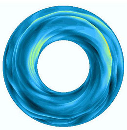
These instabilities take the form of spiral waves of the same type that occur in spiral disk galaxies such as M51, shown in the HST photo at the top of the post. In a protostellar disk, the spiral wave action pushes pulse after pulse of gas out of the regions of the disk that are in the most danger of fragmenting directly into planets. Some of this gas is forced to large distances from the central star, while the majority flows inward and eventually winds up on the star. In all likelihood, most protoplanetary disks manage to avoid direct fragmentation.

Simulation showing the development of spiral waves in a self-gravitating disk