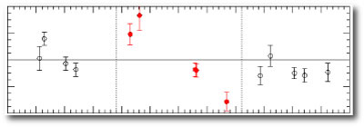
A Hot Jupiter Simulation

eggs in an egg carton

Last week, we had a one-day seminar on planets and planet formation at UC Santa Cruz that brought together researchers from both UCSC and NASA Ames. One of the talks was by Jonathan Fortney, who is currently a post-doctoral researcher in the Planetary Systems Branch of the Space Science Division at NASA Ames.

Fortney and his NASA Ames collaborator Mark Marley have a state-of-the-art radiative transfer code which can compute the emergent (and reflected) spectrum from a hot Jupiter. (See this recent post.) They’ve recently applied their code to compute how the intrinsic radiation from the flow pattern on the surface of the planet would look if you could resolve it with a pair of night-vision goggles. Jonathan writes:
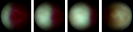
Here’s an MPEG of the full 360 orbit of HD 209458b, in 36 10-degree increments. This is as seen from Earth. It’s the Cooper & Showman (2006) dynamical simulation, run through our radiative transfer solver.

Red is 5 microns, green is 3.3 microns, and blue is 2.2 microns. The Cooper and Showman model predicts a day side that is very similar to a blackbody, leading to a whitish appearance. On the night side, which is fairly cool, strong methane absorption knocks out the blue and green, leaving only red. I have artificially pumped up the red on the night side so that you can actually see it on the monitor. If you don’t, it’s a dark red which is hard to see compared to black–the night side has little flux compared to bright (hot) day.

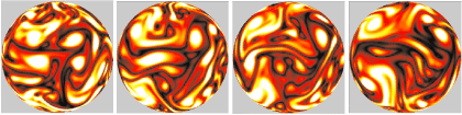
Here’s a sequence of frames from the movie:

frames from Fortney's HD209458b animation

The animation draws on calculations described by Fortney, J. J., et al., 2006, “The Influence of Atmospheric Dynamics on the Infrared Spectra and Light Curves of Hot Jupiters”, which has been submitted to the Astrophysical Journal.

This is a big step forward for the “computational imaging” of extrasolar planets, and I’m really excited about the future directions that Fortney is planning to take these calculations. For starters, it will be very interesting to see the movie with the reflected light component added in. It will also be cool to place the point of view above a particular spot on the planet and animate the time-dependant flow pattern (the above movie rotates a single snapshot model of the planet, but it does not show the actual time evolution that is computed in Cooper and Showman’s hydrodynamical simulations). Animations of the time-dependant flow will start to bring exoplanets into the territory covered by the cloud-pattern movies that the Voyager and Cassini probes radioed to Earth as they flew past Jupiter. Finally, by using John Moore’s integrating sphere to produce the actual visible colors corresponding to individual computed spectra, it will also be possible to produce true visible light (rather than night-vision-goggle infrared) animations of the simulated surface of HD 209458 b and other hot Jupiters. (In particular, HD 80606!)

Shallow Water

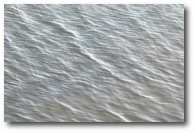
shallow water

Regular oklo readers all know that HD 209458 b is a lot bigger than it’s supposed to be.

In a previous post, we saw that the theoretical models that provide reasonable matches for the other 9 transiting planets predict that HD 209458 b’s radius should be slightly larger than Jupiter’s radius. The observations, on the other hand, make it clear that the planet is actually has a diameter about 1.35 times larger than Jupiter. HD 209458 b is by far the best-studied exoplanet, so it’s of more than passing interest to understand why it’s so large.

There’s general agreement that HD 209458 b must be privately tapping an unusual source of internal heat. Somehow, a lot of extra energy is being generated in the planetary interior. The surplus heat allows the planet to maintain an expanded outer envelope, and hence endows the planet with a larger overall size. The big question is: what is the anomalous extra heat source? A few years ago, I was enthusiastic about the idea that there might be a second companion planet that is gravitationally perturbing HD 209458 b, forcing it to maintain a slightly eccentric orbit. This eccentricity would be continually damped as a result of tidal interactions with the parent star, which would generate a sufficient amount of interior heating. Such a state of affairs is analogous to the heating of the inner Jovian satellites. The heat generated by tidal friction lends Io its off-the-hook volcanism, and maintains Europa as the Astrobiology poster world.

Unfortunately, however, the perturbing companion model no longer seems to be a viable explanation of HD 209458 b’s large size. That is, if you use the systemic console to fit to the HD 209458 b radial velocities, you’ll find that there is very little latitude for inserting significant extra planets. Try it and see, and upload your fits to the systemic back-end.

Josh Winn (MIT) and Matthew Holman (Harvard-Smithsonian CfA) have written a paper that presents an interesting hypothesis for resolving the HD 209458 b radius dilemma. Winn and Holman propose that the planet is caught in a so-called Cassini state, which is a resonance between spin precession and orbital precession. In a future post, I’ll give a heuristic discussion of the dynamics of how this situation can arise, and how the Cassini states work, but in short, if HD 209458b is trapped in the “Cassini state 2”, then its spin axis will lie almost in the orbital plane. Like all hot Jupiters, the planet will spin once per orbit, but it will literally be lying on its side as it orbits the parent star. A synchronous planet in Cassini state 2 will experience a large amount of tidal heating, even in the complete absence of any other planets in the system.

I like the Winn-Holman hypothesis because it’s potentially testable. If the planet is in Cassini state 2, then the pattern of illumination on the surface, and hence the time-dependant global infrared signature, will be very different than if it is locked into the standard upright configuration. In the standard scenario, a hot Jupiter has a fixed substellar point on its equator that does not wander significantly as the planet executes its orbit. One hemisphere of the planet is in perpetual day, while the other hemisphere experiences an endless night. Hydrodynamic calculations by James Cho and his collaborators (link), and by Adam Showman and his students (link), suggest that hot Jupiters should have a single strong equatorial jet that advects heat from the hot dayside to the cool night side. The oklo splash image has been adapted from Cho’s calculations, and shows this jet in action (see this post for more discussion).

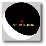
I’ve been advising UCSC Physics graduate student Jonathan Langton, who has recently begun a study of what the flow pattern on a hot Jupiter should look like if the planet is caught in Cassini state 2. If the planet’s rotation axis lies in the orbital plane, and if the planet spins on its axis once per orbit, then the play of light and shadow across the planetary orb has a pattern that is totally unlike our seasons here on Earth. At the north and south poles, of a spin-synchronous Cassini-state-2 planet, the parent star rises, passes directly overhead, and then sets once per orbit. At one special spot on the equator, on the other hand, the star is always visible, and additionally passes directly overhead once per orbit. At the opposite spot on the equator (which we’ll call the anti-stellar point), the star never fully rises, but rather peeks half of its diameter above opposite horizons once per orbit.

antistellar point

Jonathan has made two short .avi format animations that help to illustrate the situation. In the first animation, we hover above the point on the equator that receives maximum illumination. In the second animation, we hover above the point on the equator that receives the least illumination. The mythology on such a world would likely be pretty interesting.

When a spin-synchronous planet is illuminated in this bizarre manner, the flow pattern on its surface should be very different than the flow pattern that would occur if the planet is in the standard upright configuration. Jonathan has finished a preliminary set of simulations using the so-called shallow water approximation which indicate that this is indeed the case. (The shallow water approximation is a 2-dimensional method for simulating atmospheric dynamics on the surface of the planet under the assumption that the depth of the fluid is much smaller than the horizontal scales of interest. Use of this approximation doesn’t require us to assume that the red-hot Jupiter is actually covered with water!)

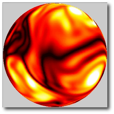
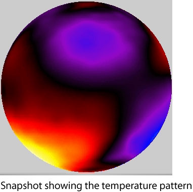
Here are two of Jonathan’s .avi format animations that show the (still very) preliminary results. The first animation [11 MB, modem users watch out!] shows the evolution of the temperature distribution (on the anti-stellar hemisphere) for a planet in Cassini state 2. Here’s a snapshot at a particular moment in time:

temperature snapshot

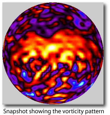
The second animation [12 MB] shows the distribution of vorticity across the planet surface. The vorticity at a particular spot in a fluid flow can be thought of as the ability of the flow to cause a tiny imaginary paddle-wheel to spin. Here’s a snapshot from the animation. The high-vorticity orange structure is a giant fiery hurricane-like storm on the surface of the planet:

vorticity snapshot

Illustrations

fan palm

I think readers sometimes wonder why oklo.org posts about extrasolar planets tend to be illustrated with seemingly random photographs from my house, my yard, and my neighborhood that bear (at best) a distant relation to the topic at hand. I’m liable to get written up on charges of pseudo-artistic pretentiousness for attempting to run the Jones Soda of Astronomy.

We’re taking this approach for several reasons. The oklo blog is designed to recruit users for the systemic collaboration, and and I’m paying the ISP out-of-pocket. An idiosyncratic format makes it easier to keep the posts flowing in the midst of the chronically never caught up academic routine of teaching, research, qualifying exams, topic defenses, homework grading, proposal writing, committee meetings, undergraduate theses, graduate advising, editing, visiting speaker hosting, etc.

Another reason is to drive home my belief that the real interest, the real fascination with extrasolar planets will ultimately lie in their tiny ephemeral details. It’s one thing to gain an abstract, theoretical understanding of the growth of planetary cores through the accretion of small bodies — it’s quite another to see a one-kilometer bolide succumb to the fiery tendrils of fluid instability as it slams into the toxic atmospheric murk of an unsettled four Earth-mass world. It’s one thing to know Neptune’s orbital eccentricity to five significant figures, it’s quite another to swoop in close to see the flow of feathered cirrus outline the turbulent core of the great dark spot.

I can’t get over the fact that I can photograph the subtly intricate details of a habitable planet available in my own backyard, and later that afternoon have them transmitted digitally across the globe. Just think, if we had an autonomous lander with a 5-megapixel camera engaged in a small-scale survey of a hectare-sized region of an Earth-mass terrestrial planet in the habitable zone of any G2V star other than the Sun, then this site would be getting a lot more than 400 visitors per day.

Finally, in resorting to the use of photographs of familiar objects to illustrate unfamiliar things, I want to underscore the urgent need for scientifically correct visualizations of extrasolar planets.

New planet-related discoveries are the subject of numerous NASA and NSF press releases and press conferences, and because these dicoveries generally report information obtained by indirect observational techniques, there’s a need for illustrations to accompany the releases “to capture the public interest”.

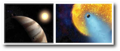
During the last ten years, these images conveying scientific results have generally been supplied by artist’s impressions. On occasion, some of these have veered toward the bizarre, the lurid, and the just plain wrong. Consider, for example, the above two illustrations of HD 209458 b. Both appeared in fairly recent HST press releases, and both are riddled with profound misconceptions. First look at that painting on the left. At the time when the image was most recently released, it was well-known that satellite orbits around the planet are highly dynamically unstable (e.g. Barnes and O’Brien 2002). The shadowing of the planet only makes sense if the star is much smaller than the planet and is somehow orbiting just above the planetary surface. The number of cloud bands and zones indicate that the planet is rotating with a ~12 hour period (like Jupiter) whereas in reality, the planet must be spin-synchronous with its P=3.5257 day orbit, and should probably have a single prominent equatorial jet. The panel on the right, which attempts to show that the planet is surrounded by an optically thin, yet Lyman-alpha-absorbing hydrogen cloud, is dramatically inconsistent with the laws of perspective, illumination, and radiative transfer. Literally billions of dollars are being spent on extrasolar planets. Surely, at the pinnacle of our dispatches, we can do better than this.

Genuinely realistic visualizations of extrasolar planets that incorporate all known information in a self-consistent way are going to become an oklo.org rallying cry over the coming year. We won’t be flying to Upsilon Andromedae any time soon. Radial velocities, photometric light curves, stellar and planetary models, dynamical integrators, radiative transfer routines, hydrodynamic codes, and Maya are what we have to work with. If it is the destiny of the extrasolar planets to truly inspire, then we must strive to see them as they really are.

Transit Fever

peppercorn on a blood orange

Literally every astronomical worker, amateur and professional alike, who has carried out a serious photometric search for planetary transits is familiar with the symptoms of at least one of the two common strains of transit fever.

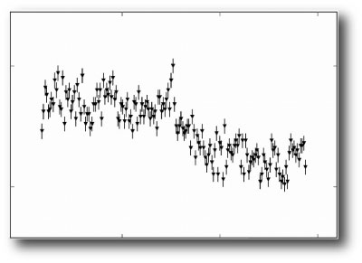
In the egressia strain, one observes a photometric time-series in which a transit seems to be ending just as the observations are starting:

egressia

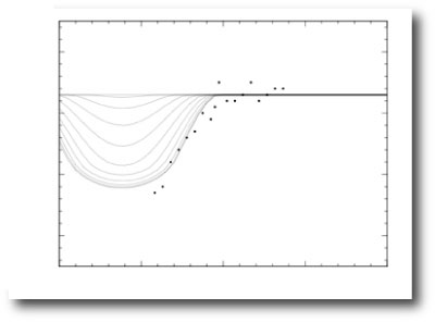
The ingressia strain has different symptoms, but is equally infectious. Near the end (or sometimes near the middle of an observing session, it appears from the time-series photometry that a planet is entering transit. In the most common form of the syndrome, the star generally either descends into the murk of high air-mass or is overtaken by dawn before the transit has finished:

ingressia

A third, somewhat rarer variety of the fever, known as rossiteria, has also been described. This strain is most commonly contracted by theorists; one finds radial velocities in the literature taken during a transit window which seem to show clear evidence of the Rossiter-McLaughlin effect:

rossiteria

I came down with my first serious case of transit fever (later diagnosed as egressia with complications due to rossiteria) nearly four years ago. The symptoms were brought on by HD 217107, the first candidate planet-bearing star observed by the transitsearch.org network. On the night of August 6th, 2002, photometric data was sent by both an observer in Pleasanton California, and from the KAIT automatic telescope at Lick Observatory. The fits to the radial velocity data indicated that the HD 217107 b transit window was scheduled to begin at 2:40 am PDT, and amazingly, both data sets showed a photometric dip right at the predicted time. To seemingly clinch the case, Debra Fisher also used the Lick 3-meter telescope to obtain five radial velocity measurements of HD217107 during and before the predicted transit ingress. When the spectra were analyzed, the velocities came back with a pattern consistent with the expected Rossiter-McLaughlin effect! [The data is available at this webpage]

To say that I was excited was an understatement. It was my first time out. I had no natural resistance. Tim Castellano, Debra, and I all came down with a full-blown case of transit fever. The period of HD 217107b is 7.127 days, which means that successive transits are spaced one week and 3 hours apart. Tim and I were on the verge of flying with a Meade LX-200 to Hawaii to observe the Aug. 13th transit from the parking lot of the Keck Observatory (That plan, fortunately, was canceled by a combination of high ticket prices and Joe Miller, the cooler-headed then-director of UCO/Lick).

By mid-September, observers in the Canary islands obtained a data set which clearly shows that HD 217107b does not transit. Huge disappointment. At that time, HD 209458 b was still the only known transiting extrasolar planet, and so the second detection would have been a very big deal.

With hindsight, having been innoculated against the transit fever, it’s clear that the transit interpretation was ambiguous in all three of our data sets. For example, in the case of the radial velocities from the Lick 3-meter, a new CCD detector for the spectrograph had just been installed, and so the overall zero point of the velocities relative to the predicted radial velocity curve was a free parameter. If the points are all moved down by 10-15 m/s, then the transit feature turns into ordinary scatter in the data. Likewise, with the photometric data, it was clear in retrospect that systematic effects were at work.

The transit detection problem is tough in part because it’s extraordinarily easy for systematic effects to seemingly conspire to produce an apparent signal. I would not feel confident in announcing a transit until I’ve seen multiple full-transit light curves. On the other hand, though, the false alarms play an important role. They get observers out on the sky, and spur the collection of enough data to truly rule out an event. This certainly wound up being the case for GJ 876, HD 168746, and a number of other candidates.

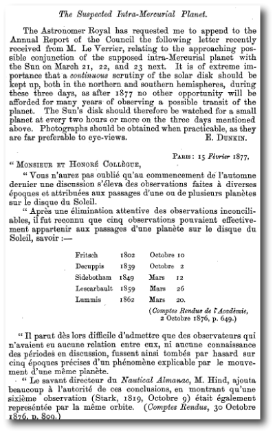
An early case of transit fever was contracted by U. J. J. LeVerrier, the Nineteenth-century French mathematician famous for the dynamical calculations that led to the prediction and subsequent discovery of Neptune. After the Neptune discovery, LeVerrier turned his attention to explaining the precession of Mercury’s perihelion, and found that the effect could be explained by the presence of a small intra-Mercurial planet that he named Vulcan. After a thorough literature search, LeVerrier unearthed five separate observations of the solar-disk transits by this planet, all at times consistent with predictions. In the following 1877 communication to the Monthly Notices of the Royal Astronomical Society, he’s basically saying, how could all those observations (which agree with theory, no less) possibly be wrong?

As everyone now knows, LeVerrier’s Vulcan doesn’t exist. The 43 extra seconds of Mercurian perihelion precession that had bothered LeVerrier so severely are explained by modifications to classical Newtonian gravity by Einstein’s general theory of relativity.

Radius anomalies?

Tristan Guillot and his colleagues have just published a paper, “A correlation between the heavy element content of transiting extrasolar planets and the metallicity of their parent stars” which explores an interesting new hypothesis for resolving the size problem for transiting hot Jupiters.

Readers of oklo.org are well aware that our theoretical understanding of the radii of hot Jupiters isn’t all it could be. For example, the transiting planets TrES-1 and HD 209458 b have very similar masses and surface temperatures, and yet HD 209458 b has a radius that is roughly 25% larger than TrES-1’s. In a previous post (see also this post), we outlined some of the hypotheses that might explain this discrepancy in radii.

Guillot et al’s idea is that the mass of a planetary core is a very steep function of stellar metallicity. That is, doubling the metallicity of the parent star leads to a 5-10 fold increase in the amount of mass contained in the cores of any short-period planets in orbit around the star. Larger core masses lead to smaller overall planetary radii at given mass, and so, in the Guillot et al. picture, planets orbiting metal-rich stars will, in general, be considerably smaller than planets of equal mass orbiting metal poor stars.

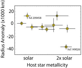
They present the following graph to support their hypothesis. It shows the difference in observed planetary size from the baseline theoretical expectation on the y-axis, and the parent star metallicity on the x-axis. They note (and the eye notes) that there is a trend in the diagram; planets orbiting metal-rich stars (as exemplified dramatically by HD 149026b) tend to be smaller than predicted, and planets orbiting stars of near-solar metallicity (e.g. HD 209458b tend to be larger than predicted.

Figure adapted from Guillot et al. 2006.

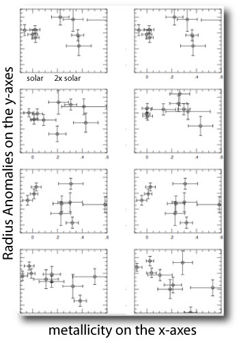
But is this correlation really present? To get a qualitative sense of whether it is or not, I took the planetary radius and parent star metallicity values for the 9 transiting planets in the Guillot et al plot and redrew them from their implied uncertainty distributions to make alternate, statistically equivalent versions of the plot in their paper. I also made control plots in which I assumed that there is no underlying radius-metallicity effect, only noise from measurement uncertainty. I made four plots of the first variety, and four plots of the second control variety. They are shown below. Can you identify which plots are the control plots?

Pantone 272

I’ve often wondered what the dayside of a Hot Jupiter would look like (with the dark, wraparound shades on, of course).

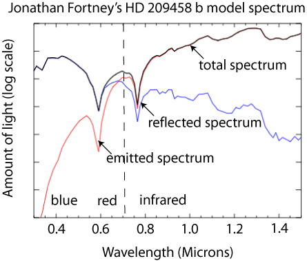
Jonathan Fortney and his collaborators at NASA Ames Research Center have been making sophisticated calculations to determine the atmospheric structures of giant planets. As a product of this research, they can compute a prediction of what the spectrum of the light coming from a short-period giant planet should be. For example, for HD 209458 b, they get the following distribution of light coming off of the planet:

If we look at the dayside (substellar point) of the planet, the total distribution of light that we would see in this model is given by the solid black curve. This total light is a sum of the light that the planet reflects (the blue line) and the light that is actually generated by the hot planet itself (the red line). As one would expect, the visible-light dayside appearance of the planet is dominated by the reflected light. The nightside image is considerably les bright, and its somewhat battered thermal spectrum is a bit more magenta than the Oklo splash image, (which was generated with a black-body color map).

Molecular absorption due largely to water and methane selectively removes yellow and green light from the reflected optical spectrum. This suggests that the hot Jupiter daysides should have some sort of purplish appearance. But what exactly will the color look like?

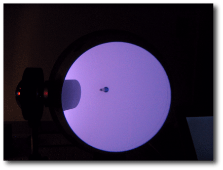
John Moores, a graduate student at the University of Arizona, and his advisor, Peter Smith, the PI of the Phoenix Mars Lander have built an optical setup which can generate (in an integrating sphere) the composite color that corresponds to any pre-specified optical spectrum. [Moores’ weblog is here]. Their goal is to obtain a source that simulates the Martian lighting environment. Given the distinctly unearthly cast to the Martian illumination, it’s of interest to see whether long-duration exposure leads to adverse psychological or even physiological effects.

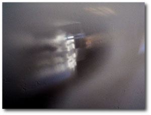
Moore used Fortney’s spectrum as an input to his apparatus to produce the image below. It shows the integrating sphere bathed in the resultant color. There is a small hole cut in the back of the sphere to allow access to a fiber spectrometer (visible as a dark spot to the left of center).

Dayside color of a hot Jupiter

To the best of our knowledge, therefore, the daysides of hot Jupiters are imbued with distinctly trendy distinctly mauve-like hues.

Good Librations

Janus and Epimetheus

Janus and Epimetheus Source: JPL

Last week, I wrote a post about the negative heat capacity of self-gravitating systems. I never cease to find it remarkable that if you drain energy out of a system that is held together by its own gravity (such as a giant planet, or a cluster of stars), then that system gets hotter. There really is such a thing as a free lunch, brought to you courtesy of the attractive gravitational force.

A collection of bodies orbiting a larger body is a self-gravitating system, and therefore will also display a negative heat capacity. We illustrated this with the idea of a satellite running through a cloud of dust. Friction between the satellite and the dust heats both bodies up, and they radiate energy away to space. The satellite simultaneously spirals into an orbit with higher velocity, and hence a higher kinetic energy, or temperature.

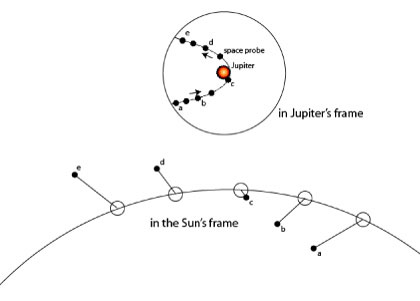
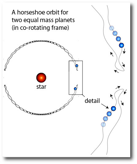
A family of orbital trajectories known as horseshoe orbits present a riff on this basic principle. A horseshoe orbit occurs when two bodies, with slightly different orbital periods, start off in near-circular orbits on opposite sides of a large central mass. The body with the shorter orbital period eventually attempts to overtake the body with the longer orbital period.

As the short-period body catches up with the long-period body, an attractive gravitational force is exerted between the pair. This force pulls the short-period body forward, and pulls the long-period body back. That is, the gravitational interaction leads to an exchange which drains orbital energy from the long-period (leading) body, and gives energy to the short-period (trailing) body. This exchange causes the bodies to swap orbital periods. The long-period body gets a shorter period, and the short-period body gets a longer period. In a frame that rotates with the average orbital velocity of the pair, the two bodies eventually come in to contact again on the opposite side of the star, and the process is repeated. Again and again in an mindlessly delicate cycle.

dynamics of the horseshoe orbit

The orbital trajectory in the above figure is lifted and adapted from a paper in the Astronomical Journal that I wrote with John Chambers. In that paper, we studied a number of weird co-orbital planetary configurations, and speculated that they might eventually be observed using the radial velocity method. If you can’t fit a particular data set with the console, the horseshoe configuration is always a good thing to check.

In our own solar system, there are two small Saturnian moons, Janus and Epimetheus, which are caught in a horseshoe-like orbit. The splash picture for today’s post shows a Cassini photograph of these moons taken near the time during which they exchange periods.

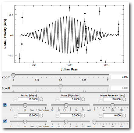
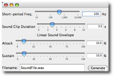
One of the most useful features of systemic console is its ability to sonify radial velocity waveforms. The soundfiles are produced by making a full integration of the equations of motion, hence all of the nonlinear gravitational interactions between the bodies are incorporated into the sound. When the console is used as a nonlinear digital synthesizer, the horseshoe orbits provide a method for producing amplitude modulation of a tone. To see how this works, launch the downloadable console, and set up the following system (just ignore the radial velocity data, since we’re not interested in fitting, but rather just in waveform generation):

console for a horseshoe orbit

That is, set up two 0.2 Jupiter mass planets with mean anomalies of 0 and 180 degrees. Make the period of one planet 10.1 days, and the other 10.0 days. For simplicity, keep the eccentricities at zero. Clicking the integration box shows the resulting radial velocity waveform. When the planets are on opposite sides of the star, their radial velocity influences on the star cancel. When they are on the same side of the star, their radial velocity influences are additive. This gives an overall modulation envelope on top of the fundamental ~10.05 day period. Use the sonify button to create a 220 hz tone out of this system:

sonifier

Here’s a link to the resulting .wav file. The amplitude modulation (or tremolo) can clearly be heard.

Try building some more complex sounds by nesting horseshoe orbits, and using unequal masses. If you get something cool, e-mail me at laughlin ucolick edu.

cleanse, fold, and manipulate

Thanks to everyone who has created an account on the systemic backend, downloaded the console, and submitted fits to the HD 69830 data sets. It’s gratifying to see the collaborative effort coming together. We’re starting to get a better understanding of which aspects of the HD 69830 data set seem secure, and which aspects are uncertain.

That outer planet seems to me to be leaning toward the latter category.

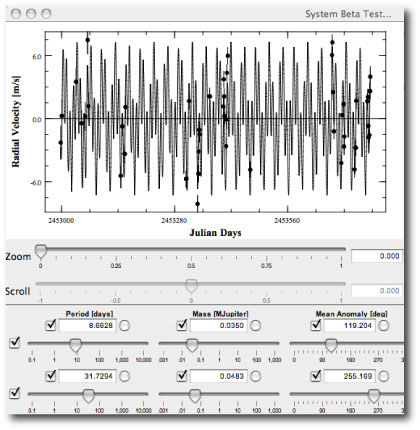
For example, I just had a look at data set #17 for HD 69830. Guided first by the console’s periodogram and then by the console’s residuals periodogram, I worked up a two planet fit to the data. I kept the orbits of the resulting 8.66 and 31.7 day planets circular. In the absence of strong planet-planet gravitational interactions or resonant disk migration, I don’t see a clear rationale for assigning non-circular orbits unless the data really demands it.

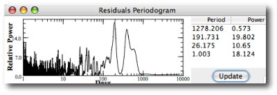
The residuals periodogram of the 2-planet fit above has peaks near 200 and 400 days. The 200 day peak is a little higher, and indeed, corresponds to the outermost planet announced in the Nature paper published last week.

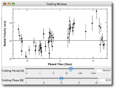
Use the folding window to look at the case for the 200 day planet. Try updating the period in tiny increments, and watch the data congeal into a relatively sinusoidal pattern. The third planet in the published fit is based on this configuration:

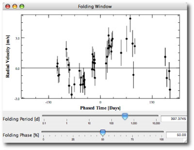
The 400 day data also looks good (although the power is not quite as high). Notice, too, that the phase coverage near 400 days is not as good. This is due both to the limited time baseline of the whole data set, as well as to the fact that the star can be observed only when it is not too near the Sun in the sky.

Apparently, the Las Vegas bookies are giving 3:1 odds in favor of the 200 day planet being correct. That said, however, the 400 day planet rounds out a very nice all-circular fit to the data.

Divide and conquer.

Hats off to everyone who’s downloaded the console, logged into the backend, and submitted fits for the HD 69830 data sets. The process now seems to be working smoothly, but we need more users. Don’t be shy! We won’t make fun of you if you turn in high-chi-square fits.

First, a follow-up note to yesterday’s post: Some of our original HD 69830-based data files did not have all their radial velocities listed in time-ascending order. This caused the periodogram generator to fail when asked to analyze these data sets. If you downloaded the console yesterday, please download a fresh copy. The version on the site now has the correctly bundled data files.

The published radial velocity data sets consist of lists of times (in Julian Days), radial velocities (relative to an average baseline velocity), and uncertainty estimates for each velocity. These uncertainty estimates give an indication of how much imprecision is introduced at the telescope and by the measurement process itself. An additional source of velocity error, generally referred to as stellar jitter, is not contained in the published uncertainty estimates. Stellar jitter is produced by various processes that are occurring on the star itself. For example, at any given moment in time, there may be a larger portion of the stellar surface upwelling than downwelling, leading to a slight, temporary, net negative radial velocity. It has generally been assumed that for a Solar-type star, stellar jitter contributes roughly 3-5 meters per second of radial velocity error, and it is certainly true that stars somewhat more massive than the Sun (Upsilon Andromedae, for example) display close to 10 meters per second of intrinsic jitter.

Recently, however, as the radial velocity observational techniques have improved, it has become clear that some stars — low mass stars in particular — can have very small intrinsic jitter. Eugenio’s analysis of the GJ 876 radial velocities indicate that the jitter in that case is almost certainly less than 2-3 meters per second. HD 69830, however, seems to be in another category altogether. The published three-planet fit suggests that the star has considerably less than 1 meter per second intrinsic jitter. If this is indeed the case, and if there are a sizeable number of stars that are as quiet as HD 69830 seems to be, then it’s clear that high-cadence observations using the RV method are destined to eventually uncover potentially habitable planets, and likely sooner, rather than later. That’s a big deal.

The twenty alternate data sets for HD 69830 have been constructed to help us test whether the stellar jitter is really as small as the fit to the actual data suggests. Some of the synthetic data sets have been produced by adopting a model in which the stellar jitter is higher than 1 m/s. It should not be possible to find fully correct chi-square ~ 1 fits to these jittery data sets. In other words if we do find chi-square ~ 1 fits to these sets, then we’ve got a strong suggestion that overfitting might be occuring in the chi-square ~ 1 fits to the real data.

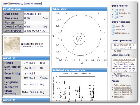
I’ll wrap up today with a set of screenshots showing how the backend environment operates. The best way to learn how it works, however, is to login and start using it. It’s quite self-explanatory.

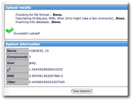
After you’ve uploaded a fit from your own computer, you’ll get a response page that looks like this if the upload was successful:

Make sure that your fit file is appended with the suffix “.fit” before you upload it.

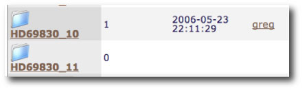
If you click on “view systems”, you’ll see a list of all the systems that have been added to the console thus far. All of the fits that have been uploaded by the systemic collaboration can be accessed from this catalog page. As of tonight, most of the systems have not yet been fitted…

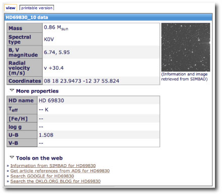
Clicking on a system name brings up the corresponding system data page. There’s quite a bit of information available:

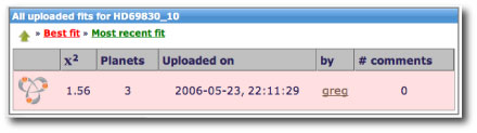
If you click on the icon next to a particular fit:

Then information about the planetary system corresponding to that fit is displayed:

Let’s see some activity! These planets won’t fit themselves…

Time for work!

I think we’ve finally got the pieces in place. Its time to really push the collaborative aspect of the systemic project. (1) Aaron’s downloadable console has been tested, updated, and is known to work on Mac, Linux, and Windows platforms. (2) Stefano’s systemic back-end collaborative space is tested and working. (3) Eugenio and Paul are standing by and ready to provide technical support. (4) We’ve got nearly 400 unique users visiting oklo.org every day, and (5) with HD 69830, we have an extremely interesting new system to subject to the analytical and computational power of the distributed oklo community.

The questions to be answered are (1) is the published HD 69830 fit unique? and (2) can we get an independent estimation of the errors?

To get an initial analysis of these questions, I’d like to invite (and encourage!) the oklo community to use the console and the back-end environment to obtain a wide variety of fits to a new set of 21 radial velocity datasets. These data have been uploaded onto the web-based console, and they are also packaged into an updated version of the downloadable console. The data sets include the published HD 69830 data, along with 10 bootstrapped datasets, and 10 model-based synthetic data sets. I’ll write much more about bootstrapping and synthetic data sets in upcoming posts. For the time being, we’re simply interested in finding a variety of fits to these data.

The rest of this post will take the form of a brief tutorial to get you going. We really need as many people as possible to participate in this effort.

First, download the console onto your computer. The link to the downloadable console on the right menu bar gives download instructions. If you’re using a non-US English character set on a Windows machine, you will need to switch to the US English set. (We’ll have a fix in for this shortly.) Launch the console on your computer.

Note that the console application, “systemic.jar” is contained in a directory (folder) that contains several subdirectories. These subdirectories are named “datafiles”, “fits”, and “soundClips”:

When the console is running, select one of the HD69830 data sets from the system menu, and obtain a fit. Once you’ve got the fit, use the “save” button (a new feature of the downloadable console) to save the fit in the “fits” directory. Use the suffix “.fit”, as shown below:

Next, point your web-browser to the systemic back-end. The full url is: http://www.oklo.org/php/login.php

You’ll see the login page. Register as a new user. Once you’re logged in, the environment is designed to be as self-explanatory as possible. In particular, you can upload your fit from your computer, and compare it with other users’ fits to the same system. Go ahead and explore! The back-end contains a number of very interesting features, which we’ll look at in the next post.

20 centimeters per second

tubeworms

Source: Nicolle Rager Fuller NSF


HD 69830
. What a difference a year makes. Last June, HD 69830 languished in the obscure backwaters of the Henry Draper Catalog. Now, however, like its buddy HD 209458, the star is a star. Google “HD 69830”, and the search returns 660 entries (and growing daily). Google “HD 69831” and (until the crawlers manage to find this post) your search does not match any documents.

In Thursday’s post, we gave an overview of the HD 69830 planetary system, which contains Neptune-mass planets in 8.67, 31.6, and 197 day orbits. Perhaps the most astonishing thing about this discovery announcement is the tiny radial velocity amplitude of the 197 day planet in the model. This object induces a radial velocity amplitude of 2.2 meters per second, with a reported error of only twenty centimeters per second. That’s about the speed your finger moves if you trace it quickly across the title of the discovery paper. This detection required a very quiet star and an extraordinary technique. The Swiss seem to have broken through to the next level.

I wonder what that outer planet looks like. Over at transitsearch.org, I have a Fortran cron job that processes all of the known exoplanets every night to produce updated transit ephemeris tables. In order to predict transit depths, the code needs an estimate for the planetary radius, which in turn requires an estimate of the effective surface temperature. The transitsearch model reports 262 K, just below the freezing point (273 K), suggesting a brilliantly reflective orb swathed in white water-based clouds.

In an upcoming post, I’ll delve into some responsible (and also some irresponsible) speculations about the world beneath those clouds. A responsible viewpoint has planet “d” forming at a larger orbital radius than it currently occupies, and then migrating in to position. In this formation-followed-by-migration scenario, there were plenty of ices available during planetary assembly, and the planet will have a structure (and size) very close to those of Neptune.

internal structure of HD 69830 d

An irresponsible, more provocative scanario has planet d forming in-situ, out of refractory silicate and metallic materials. The final product in this case is a super Earth, smack in the sweet spot of the habitable zone, and endowed with ten Hubble times worth of geothermal activity. But more on that in the upcoming post.

A driving goal at oklo.org is to get our readers beneath the headlines and critically examining what the radial velocities themselves have to say. To do this, we need the data. The Lovis et al. discovery article in Nature contains a link to supplementary material, but when you click on the link you get a .pdf article about hydrothermal vent tubeworms:

huh?

Hmmm. Even if we adopt the most optimistic giant-Earth-like structural models for HD 69830 d, this supplementary material seems to be jumping the astrobiological gun. With tubeworms obscuring the radial velocities, we were compelled to resort to Dexter to extract as many velocities as we could from Figure 2 of the .pdf version of the paper. Eugenio managed to scrape 53 data points off the graph. We were busy using the console to work up fits to these dextered velocities when Darin Rogozzine at Caltech managed to guess the correct link and supplied oklo.org with the url.

In the next post, we’ll have a go at the rv’s. If you want an advance crack at them, they’re now on the web-based version of the console. We’ll get them on the downloadable version tomorrow.

XO-1

Image source: designonline.se

Today’s astro-ph mailing contains a paper by McCollough et al. detailing the discovery of a new transiting planet orbiting a sun-like star lying in Corona Borealis. Dubbed “XO-1” — easily the coolest name yet for an exoplanet– this world has a year that lasts 3.941534 days, and a mass roughly 90% that of Jupiter. The temperature at the scalding, toxic, vortex-riddled cloudtops should be a torrid 1083 K. It ain’t no habitable world, folks, but as the fifth extrasolar planet found to transit a relatively bright (V=11) parent star, it’s big news nonetheless. Bright parent stars are great for planetary characterization, because they make detailed follow-up a lot easier to carry out.

The preliminary indications are that this planet, which has a measured radius of 1.3 plus or minus 0.1 Jovian radii, is somewhat larger than expected. Our theoretical models predict that XO-1 should have a radius of 1.05 Rjup if there’s a 20-Earth mass core, and 1.11 Rjup if the planet is core-free. If the large radius is confirmed, then we’ll be faced with the same radius problem that we’re facing with HD 209458 b (as explained in this oklo post from Dec. 2005). An interesting clue may be provided by the fact that the XO-1 parent star, like HD 209458 is not particularly metal rich.

The paper lists four amateur observers as co-authors. Three of them, Tonny Vanmunster, Ron Bissinger, and Bruce Gary, are long-time transitsearch.org participants. P.J. Howell is the fourth amateur co-author on the list. As usual, the photometry that these guys are getting is excellent:

amateur lightcurves of XO-1

Figure adapted from the McCollough et al. paper.

The paper describes in detail how the photometry from the amateur observers was able to effectively leverage and speed up the discovery, and how the ready-made network provided by the small-telescope observers eliminated the need for an expensive robotic follow-up observatory.

Sounds to me like it’s time to crack open a bottle of Hennessey XO. Congratulations all around, guys!

Three Neptunes

The published census of extrasolar planets grew by 1.57% today, with the Geneva Extrasolar Planet Search Teams’s announcement in the journal Nature that trois Neptunes orbit the nearby sunlike star HD 69830.

There are a number of reasons why the Swiss team’s paper is interesting. The HD 69830 system seems tailor-made for a detailed dissection with the Systemic Console. This dissection can get the oklo user-base up and running with the new beta version of the Systemic Backend. In addition, the configuration of this system has some fascinating consequences for the theory of planetary formation and evolution. It is definitely worth digging into this story for the next few posts.

First, the nuts and bolts of the announcement. The three planets, named — you guessed it — HD 69830 “b”, “c” and “d”, clock in with Msin(i) estimates of 10.2, 11.8, and 18.1 Earth masses respectively. Assuming that the system is co-planar and is being viewed close to edge-on, this places b and c squarely in the mysterious planetary mass range that falls between the ice giants (e.g. Uranus and Neptune) and the familiar terrestrial planets. Planet d is somewhat more massive, with a net bulk almost exactly equal to that of Neptune. [It’s important to remember that the inclination of any given planetary systems is more likely to be viewed edge-on (i=90 deg) than pole-on (i=0 deg) for the same reason that the Earth has more real-estate within a hundred miles of the equator than within a hundred miles of the poles.]

Orbits of HD 69830 b, c and d

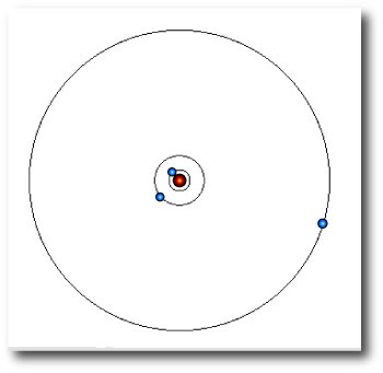
The published orbits of HD 69830’s planets are, however, distinctly unreminiscent of Uranus and Neptune. HD 69830 b orbits in 8.667 days, c orbits in 31.6 days, and d circles the star once every 197 days. All three have modest eccentricities.

For kicks, here’s a .wav format sound file which turns the reflex radial velocity waveform from the star into an audio signal. [Note: you can use the downloadable version of the Systemic Console to produce an audio representation of any planetary system, see this post from last week for the details.] In the sample file for HD 69830, I’ve pitched the innermost planet to a rather piercing 3 octaves above A 440. The period difference betwen the inner and outer planets leads to ~4.5 octaves of pitch difference. Planet d’s contribution can be heard as a bass drone about 2 octaves below middle C.

Indeed, the “chord” produced by these three new planets sounds terrible. Badly out of tune, to be precise. This immediately tells us that ther are no strong mean-motion resonances in the published configuration of planets. The human ear-brain system is good at on-the-fly calculation of whether the mean-motion resonance arguments are in circulation or libration. For example, this .wav file corresponds to a (synthetic) planetary system that is participating in several mean-motion resonances. When compared to HD 69830, it sounds awfully good.

As soon as I saw those periods — 8.667 days, 31 days, 197 days — I raced ahead through the paper draft to see if a photometric check for transits was carried out already by the discovery team… Excellent! There’s no mention anywhere in the paper of an attempt at a photometric search for transits of the planets. This will lend a challenging, high-profile opportunity to transitsearch.org. My guess is that the Geneva team was quite eager to get these three worlds out the door, and did not want to hold up the show with an exhaustive photometric check. There’s a real danger that you’ll wind up getting scooped if you cross all your photometric T’s before publishing your radial velocity-detected planets.

In the next post, we’ll look at what the radial velocities have to say.

Negative Heat Capacity

hydrodynamic turbulence in a keplerian disk

Imagine leaving the front door open on a cold day, and having the inside of your house grow warmer as a result. Curiously, that’s exactly how self-gravitating systems such as stars, nascent giant planets, accretion disks, and globular clusters behave. Drawing energy from any of these systems causes them to heat up. The negative heat capacity of self-gravitating systems is one of the most central concepts in astrophysics.

The dynamics of the Keplerian orbit can be used to understand how this works. Imagine a particle initially on a circular orbit around a central star. The particle slams into a cloud of dust. As a result, the dust and the particle both heat up and radiate energy. The particle decreases its velocity and drops into an eccentric orbit with a smaller semi-major axis.

particle going through a cloud

Here’s the key point: the smaller semi-major axis means that the average squared speed of the particle (averaged over an orbit) has increased. The fact that the particle is slow near apastron is more than compensated by the high speed near periastron. Since the particle’s kinetic temperature is proportional to its speed squared, the temperature of the system goes up. In effect, the reserve of gravitational potential energy gets double billed: once to provide the radiated energy, and a second time to increase the kinetic energy of the particle.

It’s a lot like taking a cash advance on your credit card and using half to pay late bills and the other half to buy a set of 22 inch rims for your Escalade. It’s a little sad to observe Nature operating on such a dissolute and spendthrift principle.

backend

Bertinoro, AGN and galaxy

Hey all! This is Stefano, one of the Systemic team members. I’m an MSc astrophysics student at the University of Bologna, Italy, and will be transferring to the beautiful city of Santa Cruz next year to start working on PhD.

I just came back this evening (18 pm on the West coast) from the National School of Astronomy, Bertinoro, where I’ve been sent to last week. It takes place in an old little city, surrounded by walls and dominated by a castle. The castle has bedrooms and seminar rooms with frescoes and red carpets. I was sleeping IN the castle, when I woke up I could see the green planes of the pianura padana extending for acres and acres, and little rocky houses of farmers. The city is famous for its wine. Galla Placidia, daughter of the Roman emperor Theodosius, drinking a glass of the sweet white wine albana purportedly said to the wine “sei degna di berti in oro” (you deserve to be drank in a golden glass), from which the name of the city “Bertinoro” comes. The city itself is full of little places to drink wine (the amazing Sangiovese) and other kinds of alcoholic beverages, which of course we visited often, more than once a night! Whoever thinks scientists are grey, sad people should have come to one of these crazy nights.
That said, it was my first astrophysics school, and I felt so young and unexperienced! Everyone was working on their PhD, and was brilliant, accomplished, and just plain cool — at least to my eyes. I was feeling really out of place in the midst of these amazing minds talking about galaxies and AGNs citing models and theory with apparent ease.

Thankfully I soon realized that these scientifical “hierarchies” don’t really stop you to have your say and give your, even small, contribution! And anyone, from a last-year student like me to the famous astrophysicist, is collaborating in an amazing community to help develop our knowledge of where we are and what’s been before us.
The astronomer Edwin Hubble
All this to introduce the systemic Backend. The systemic Backend lets you have your say in the field of extrasolar planets!

Thanks to the systemic console, you can fit radial velocity data taken by real astronomers and as easily as possible try to discover the evidence of unseen planets around distant stars. And it doesn’t matter if you’re an astronomer, an high school student or an astrophile out of budget for a telescope: if your findings are consistent with the data and explains the observations better than before, you’ve done it!

The systemic backend lets you share your results with other enthusiastic people, showcase your results and interact with your fellow colleagues, just as you would do on a myspace-like network. You can upload the fits saved from the console online from your account, and have other people enthusiastically comment or bash your findings. You might be doing real astrophysics, while knowing other people.

Try out the beta version of the system now, help us iron the bugs and the improvements to make!

The systemic console and backend will be part of a bigger picture — Greg will be talking about it in a future post.

More soon,
Ste