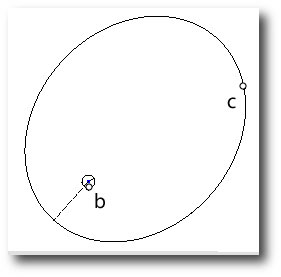
data data data

mirror in the boardwalk please talk free

Saturday was an epic day for the radial velocity consuming public. Paul Butler and the California-Carnegie planet search team published a blockbuster paper in the Astrophysical Journal, and it looks like the first weekend’s gross is gonna be huge. The paper announces the detections of five new planets, and publishes re-analyzed and (in many cases) greatly expanded radial velocity data sets for no less than eighty three planet-bearing stars. The velocities are all available in machine-readable tabular form. No dextering, no unfolding, no typing, no postscript extractions. As an added plus, the paper also provides the latest estimates for jitter, mass, metallicity, and vsin(i) for all of the tabulated stars.
Needless to say, there’s a great deal of interesting data in this compendium. The updated 55 Cancri velocities, for example, should aid the characterization of a fully self-consistent model of that system. The slew of fresh velocities will be of great help in constraining the uncertainties in the transit predictions for planet bearing stars.

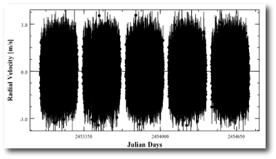
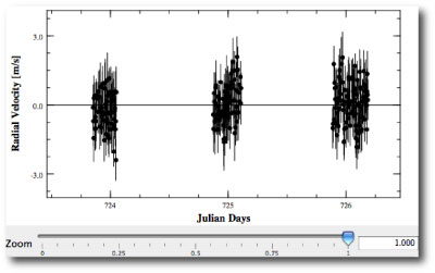
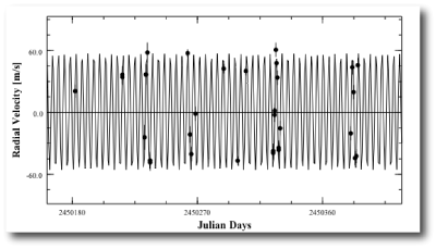
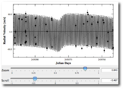
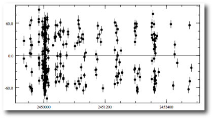
I dug right in to see how the 51 Peg system (described in a series of posts detailed here) is holding up. There are now 256 new and updated velocities from Lick Observatory to complement the 153 published Swiss velocities. The time-series shows a well-sampled mixture of long-term cadence and intensive monitoring.

all the 51 peg velocities

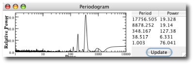
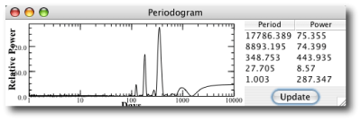
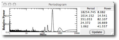
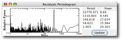
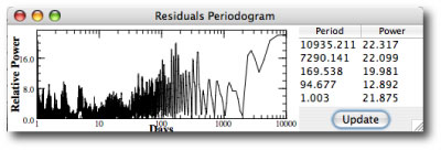
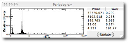
Needless to say, 51 Peg b is still present with a vengeance. The power spectrum of the combined 409-point data set has a certain overwhelming 4.231 day character:

power spectrum of all the 51 peg velocities

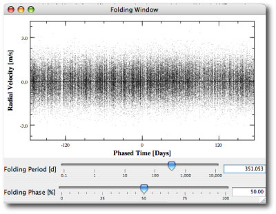
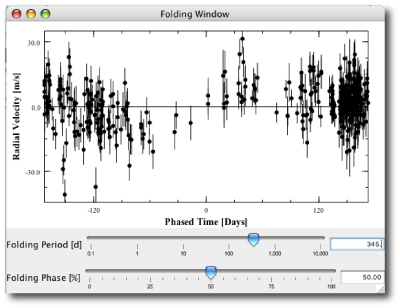
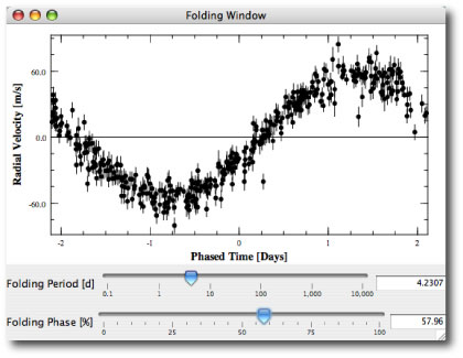
The data set phased at 4.2307 days shows a very nice sinusoid. About a thousand orbits have been folded down to make this plot:
all the 51 peg velocities folded together

So how does 51 Peg “c” fare in the new dataset? I’ll post an analysis tomorrow. If you’re impatient, though, you can use the downloadable console to investigate what the new data has to say.

extraterrestrial

thistle against a white background

Image Source

We’re working hard to keep the systemic project moving forward.

Eugenio, as of July 14th, has compiled and documented all of the published radial velocity data sets, and has been designing and developing the “KeckTAC” code, which will be a workhorse for systemic’s next phase. The published datasets are all available on the systemic systems catalog. Aaron has stripped the console down to its component parts, and he’s rebuilding it with new features, faster algorithms and a sleekly expandable architecture. Stefano has been tweaking the systemic backend [sign up and get fittin’, y’all -ed.], and will be arriving at UCSC in the Fall to do his Ph.D. research. We’re hoping that part of his thesis will be a statistical analysis of the final results of the 100,000 star systemic simulation.

When I was in graduate school, I spent a lot of time doing research on brown dwarfs (objects between 13 and 75 Jupiter masses that lie in the mass range between giant planets and red dwarf stars). At that time, circa 1992, no bona-fide brown dwarfs had actually been found, but the prospects for detecting them seemed reasonably good. My friend Todd Henry, who was a graduate student at the University of Arizona, and who was hunting for brown dwarfs using the speckle method, told me something that stuck in my mind.

“Face it, Greg,” he said, “the reason you’re interested in brown dwarfs is not because you’re interested in Brown Dwarfs — the reason you’re interested in brown dwarfs is because you’re really interested in planets, and brown dwarfs are just one stop away on the line.”

He was right.

A similar logic might apply today, “The reason I’m interested in giant planets is not because I’m really interested in Giant Planets — the reason I’m interested in giant planets is because I’m really interested in habitable terrestrial planets, and giant planets are one stop away on the line.”

Pollux

Image Source.

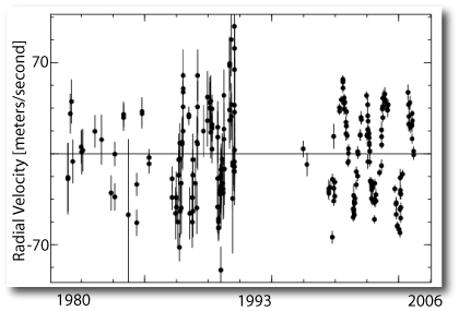
Several weeks ago, the planet count at the extrasolar planets encyclopedia notched up by one with the announcement by Artie Hatzes and his collaborators that Pollux (Beta Geminorum) is accompanied by a ~2-3 Jupiter mass planet on a 590 day orbit. This world has been under construction for a long time. The first published radial velocity data point for the star dates back to Nov. 15th, 1980, and Hatzes et al. brought 55 new radial velocities to the table to seal the detection. The planet was independently confirmed by Reffert et al., who (in a preprint posted July 7th) deliver an additional 80 high-precision velocities.

velocities for beta gem

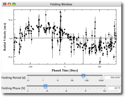
All told, there are now seven published datasets, and all are available on both the on-line and downloadable versions of the console. When folded together, at a 593 (1.6 year) period, a full quarter century’s worth of radial velocity data show the planet quite nicely.

After the Sun, Pollux is the 17th brightest star in the sky. It’s prominently visible both because it’s close (34 light years) and also because it’s an intrinsically bright K0III giant star. Pollux is about 1.9 times more massive than the Sun, and is already coming to the end of its life. It has left the main sequence, and is beginning its long trek up the red giant branch of the Hertzsprung Russell diagram.

In last Saturday’s post, I wrote about predictions of the core-accretion hypothesis with respect to planet formation. The ability to quickly build a Jovian-mass planet depends on the surface density of solid material in the protostellar disk. A lot of solids leads to rapid buildup of cores, and hence the ability of planets to achieve rapid gas accretion before the protostellar disk dissipates. (The spiral wave-induced evolution of marginally gravitationally stable disks leads one to expect that disk masses will correlate with the masses of the central stars, see this paper for a lot more discussion.) All other factors being equal, one expects that Jupiter-mass planets will be rarer around stars that have significantly less mass than the Sun, and that conversely, Jupiter-mass planets will be more common around planets of somewhat higher mass than the Sun. (Note that for really massive stars, the luminosity of the star itself will rapidly photo-evaporate the disk, which will cause problems for giant planet formation via core accretion).

Unfortunately, it gets increasingly harder to apply the radial velocity detection method to Main Sequence stars that are considerably more massive than the Sun. The higher temperatures of these stars lead to weaker spectral lines. Weaker spectral lines make it hard to get really accurate radial velocities. Higher mass stars also tend to be fast rotaters, which further smears out the lines, and they are often subject to pulsations which can mimic the radial velocity signature of an orbiting planet. Above about 1.3-1.4 solar masses, it thus becomes hard to survey main sequence stars for planets.

Luckily, however, a trick can be used to assess the planet frequency for high-mass stars. As a star that has ~1.5-3 solar masses ends its main-sequence hydrogen burning life, its core begins to contract and its outer layers swell up and cool down. The atmosphere of the star then regains the wealth of spectral lines that can be used to make accurate radial velocity measurments, and hence detect planetary companions. The core accretion theory predicts that planet hunting around such giant stars should be a highly profitable enterprise.

The sand reckoner

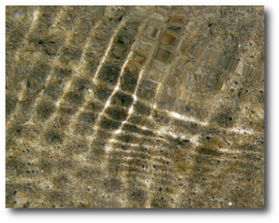
shallow water caustics

Image source.

Four out of five astrophysicists surveyed recommend the core-accretion theory to those interested in planet formation theories.

Oklo regulars know that I lean toward core-accretion over gravitational instability as an explanation of the dominant mode of planet formation. I think that core-accretion does a superb job of explaining the planet-metallicity connection, and I don’t think that the initial conditions that underlie hydrodynamical calculations that show disk fragmentation are physically realistic.

The key aspect of core-accretion is that it is a threshold phenomenon. If a planetary core reaches a Neptune-like mass of ~10-20 Earth masses while there is still gas in the protoplanetary disk, then it will rapidly accrete that gas, and (in most cases) increase its mass by a factor of ten or more. On the other hand, if a core reaches a Neptune mass after the gas is gone, then the growth will cut off, and the core will end its days as a modest ice giant.

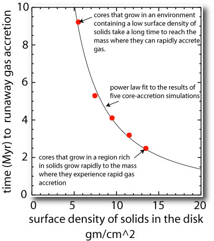
The amount of time that it takes for a core to reach the phase of rapid gas accretion depends sensitively on the amount of solid material that is available in the disk in the form of planetesimals. A disk with a high surface density of solids is capable of rapidly assembling a core, thereby forming a Jovian-mass gas giant quite quickly. Recent simulations suggest that an average protostellar disk surrounding a star of solar metallicity will lie right at the threshold of being able to manufacture a Jovian planet. This result gives a satisfying mesh with the observations. As stellar metallicity exceeds solar, the fraction of stars with detectable Jovian-mass planets increases very rapidly. Disks that form their Jovian planets early-on are better able to migrate them into the terrestrial region where they can easily be detected. Stars of solar mass and metallicity will tend to have giant planets that remained, like Jupiter, more or less where they formed. Stars with subsolar metallicity will rarely be accompanied by Jupiter-mass planets.

time to formation of a jovian planet as a function of surface density

In addition to explaining the planet-metallicity connection, core-accretion provides a number of other testable predictions. Our simulations suggest that a growing planet orbiting a star with 40 percent of the Sun’s mass will require more than 10 million years to “go Jovian.” After 10 million years, however, the gas in most protostellar disks is long gone. The core-accretion theory predicts, therefore, that low-mass red dwarf stars should very often be accompanied by Neptune-mass planets but should almost never have Jupiter-mass companions.

The surface density of solids in a protostellar disk is correlated with metallicity, and some heavy elements are more important than others. Oxygen, for example, in the form of water ice, is of fundamental importance for building cores. At given mass and overall metallicity, therefore, a disk that is naturally rich in oxygen should be better able to form Jupiter-mass planets. Silicon-rich disks too, should have an enhanced capacity for building gas giants.

208 nights, please

life on alpha Cen Bb

image source

The data from the Hipparcos satellite indicate that it’s very likely that Proxima Centauri is in orbit around Alpha Centauri. Proxima has not simply been caught in the midst of a stellar drive-by. It’s cool, certainly, that our nearest stellar neighbors are going along to get along, but is there any scientific importance in the fact that Proxima and Alpha are gravitationally bound?

The answer to this question is a definite yes.

If Proxima is in orbit around Alpha, then we can safely assume that the three stars formed together from the same giant molecular cloud. Therefore, all three have the same age and metallicity. Alpha Centauri A and B, furthermore, are among the best-studied stars in the galaxy; a query to Simbad on Alpha Cen returns a cool 311 citations during the 1983-2006 timeframe. The fact that they are so close and so bright means that very detailed and accurate models can be made of their properties. It’s been clear, for example, since the early 1970s, that the stars are more metal-rich than the Sun. The most recent determination (by Jeff Valenti and Debra Fischer) puts the metallicity at 0.19 “dex”, or 150% of the solar value. Other recent studies suggest even higher metallicities. A detailed modeling study by Eggenberger et al. 2004 finds an age for the stars of 6.52 billion years (plus or minus 300 million years). Proxima was 2 billion years old when the Sun and Earth formed, and it will outlast the Sun on the Main Sequence by 5 trillion years.

Metallicities for red dwarf stars are notoriously difficult to determine. Low-mass red dwarfs are cool enough so that molecules such as titanium oxide, water, and carbon monoxide are able to form in the stellar atmospheres. The presence of molecules leads to a huge number of lines in the spectra, which destroys the ability to fix a continuum level, and makes abundance determinations very difficult.

Recent progress on the red dwarf metallicity problem has been made by Bonfils et al. (2005) who employed a clever approach. They use the fact that when a red dwarf is a member of a multiple system (like Proxima) in which the primary star is more massive, then the metallicity of the red dwarf can be induced by measuring the metallicity of the primary star. Bonfils et al. found 20 nearby binary pairs where this trick was possible, thus giving them the metallicities of 20 red dwarf stars. They then developed an empirical metallicity calibration for red dwarfs based on easily measured photometric indices. Using this technique, they were able to estimate that GJ 876 has a metallicity of +0.02 dex, very close to the solar value. (The fact that GJ 876 is not particularly metal-rich makes one wonder how it managed to put together such an off-the-hook planetary system, but that’s a different topic.)

With Proxima bound to Alpha, we know that its metallicity is ~0.2 dex, which will provide a very important new point of improvement for calibrations based on the Bonfils et al. technique. Of the 20 stars in the Bonfils calibration, only five were above solar metallicity, and only one (GL 324) is as metal-rich as Proxima. Looks like Proxima has provided yet another opportunity for a class project for this Fall.

Just about everyone wants Alpha Centauri to harbor habitable planets. The fact that Proxima is gravitationally bound to Alpha will help make this a reality.

Given what we know about planet formation, it’s extremely likely that there are terrestrial planets in orbit around both Alpha Centauri A and Alpha Centauri B. Simulations by Wiegert and Holman (1997) show that the habitable zones of both planets are likely dynamically stable. Elisa Quintana and her collaborators (2002) have carried out accretion calculations that indicate that terrestrial planet formation should proceed very easily around both stars (with 3-5 terrestrial planets expected for each). Because the metallicity of Alpha Centauri is higher than the Sun, the naive expectation is that these planets should contain of order two times as much mass as our own terrestrial planets.

At first glance, one expects that the Alpha Centauri planets will be very dry. The period of the AB binary pair is only 79 years. The orbital eccentricity, e=0.52, indicates that the stars come within 11.2 AU of each other at close approach. Only refractory materials such as silicates and metals would have been able to condense in the protoplanetary disks around Alpha Centauri A and B. To reach the water, you need to go out to the circumbinary disk that would have surrounded both stars. With only A and B present, there’s no clear mechanism for delivering water to the parched systems of terrestrial planets.

Enter Proxima. With its million-year orbit, it has gone around Alpha roughly 6500 times. The periodic perturbations induced by its close approaches will dislodge comets from the outer circumbinary regions, and send them sailing in to smack the terrestrial planets, delivering the much-needed water and mass-extinctions. Detailed simulations need to be done to look into this process (yet another Proxima-inspired class project).

I’m willing to bet a hundred dollars that the Alpha Centauri Ab and Bb exist, and that these planets are reasonably close (or inside) the habitable zones. How can we confirm the existence of these planets?

The spin axis of Alpha Centauri A is aligned with the angular momentum plane of the AB binary, which indicates that the planets will almost certainly orbit relatively close to the binary plane as well. The binary plane is inclined by 11 degrees with respect to our line of sight (79 degrees with respect to the plane of the sky) and so transits are a long-shot.

What about radial velocities? For sake of example, let’s assume that there’s a 2 Earth-mass planet in a habitable orbit around Alpha Centauri B. The habitable zone for B lies at 0.75 AU, which corresponds to an orbital period of 250 days. Assuming a circular orbit, and adopting and i=79 degree orbital inclination, the radial velocity half-amplitude is 10.6 centimeters per second.

In a series of posts in May, I looked in detail at the Swiss discovery of three Neptune-mass planets in orbit around HD 69830. These detections were based on 74 high-precision radial velocity measurements of a K0V star that is essentially identical in age and mass to Alpha Centauri B. HD 69830 “d”, the most distant planet in that system, induces a half amplitude of K=220 cm/s, with an error of 19 cm/s.

Given that HD 69830 d was detected with 74 measurements, Poisson statistics indicate that 484 times more observations will be required to detect our putative 2-Earth mass Alpha Centauri B “b” with a similar level of confidence. That means 35,816 RV data points, which means 35,816 individual spectra, which is a lot.

Surprisingly, however, such a program is not totally outside the realm of possibility. Because of its extreme proximity, Alpha Centauri B is a bit more than 100 times brighter in the sky than is HD 69830. This means that for a given signal-to-noise, a spectrum for Alpha Centauri B can be obtained 100 times faster than a spectrum of HD 69830. The crucial limiting factor to obtaining observations of Alpha Centauri B will be the readout time for the CCD. If I am interpreting the HARPS instrumental web pages correctly, this readout time for a high-resolution spectrum is 197 seconds (if someone is in the know on this, please post a comment). A reasonable observation cadence, then, seems to be about 210 seconds per observation, meaning that Alpha Cen B b can be detected on HARPS using 208 dedicated 10 hour nights.

A Million-Year Picnic

Amusement Park Ride, Santa Cruz Beach Boardwalk

Image source.

Last week, I wrote about a plan to send a tiny spacecraft on a trip to the vicinity of Alpha and Proxima Centauri. The idea is to employ a multi-stage rocket to boost a tiny payload toward the stellar system at high speed. When the destination is reached, the principle of gravity de-assist (in the form of successive close flybys of the stars) is used to haul the spacecraft into a bound orbit without using any on-board fuel. [This, of course, is an exercise in orbital dynamics, and not mission proposal. There are better ways to get to Alpha Centauri.]

The problem was tackled by UCSC graduate student Jeremy Wertheimer as his term project for my Astrophysical Dynamics class. Our initial plan was to use a multiparameter minimization scheme (such as the genetic algorithm or simulated annealing) to vary the incoming trajectory of the spacecraft until we found the largest arrival speed that allows for a final bound orbit. To do this requires us to have a precise orbital model for the Alpha AB — Proxima trio.

Amazingly, we discovered that the most recent papers in the literature (from the early 1990s) had arrived at the conclusion that Proxima Centauri is not bound to the Alpha Centauri binary, but rather is in the process of merely drifting past them like a ship in the night. The a-priori odds of Proxima being so close, and so nearly bound, are less than one in a million, but nevertheless, the best position and velocity measurements at that time suggested that this was indeed the case.

In the intervening years since the Matthews & Gilmore 1993 and Anosova et al. 1994 Proxima-Alpha papers were published, there has been a tremendous improvement in our knowledge of the positions, distances, and space velocities of the nearby stars. This improvement is largely due to the European Space Agency’s Hipparcos astrometric satellite, which flew between November 1989 and March 1993 (and whose data was published in June 1997). Hipparcos obtained excellent 3D positional and plane-of-the-sky velocity measurements for both Alpha and Proxima Centauri. When combined with mass and radial velocity measurements for the three stars, the Hipparcos data allows a much better determination of the orbit.

When Jeremy computed an orbit for Proxima using the updated Hipparcos data, he discovered that the measurements now suggest that Proxima Centauri is just barely bound to the Alpha AB pair. He found an enormous elliptical orbit with semi-major axis 272212 AU. (This works out to a whopping 4.3 light years, which is coincidently quite close to the current Sun-Proxima distance.) Clearly, this orbit is much too large, but it’s encouraging to see that the centroid kinematic measurements now indicate that Proxima is formally bound to Alpha.

Even the latest measurements for the Proxima-Alpha Centauri positions and velocities contain uncertainties. In particular, it turns out that the absolute radial velocity for Proxima Centauri has a (still surprisingly large) 1-sigma uncertainty of 200 meters per second. Proxima’s radial velocity in turn has an important effect on whether the three stars are gravitationally bound. Jeremy ran a Monte Carlo simulation in which he drew 10,000 models of the Proxima-Alpha system parameters from the Gaussian distributions implied by the uncertainties in the observations. When he plots the binding energy of these models against the value for Proxima’s radial velocity, he finds that 44% of the trial systems are bound (that is have total energy = gravitational energy + kinetic energy less than zero).

Monte Carlo simulation for Proxima Orbit

Many of the bound trial systems have energies very close to zero, and hence place Proxima in absurdly large orbits around Alpha. In these configurations, Proxima is currently at the periastron (that is, the near-point) of its orbit. An object in a highly eccentric orbit, on the other hand, spends most of its time near apastron (the orbital far-point).

To illustrate how objects tend to spend their time near apastron, here’s a home-made mpeg-4 stop-action animation of a peppercorn orbiting a kumquat in an ellipse with e=0.90. (Try this version if the other one loads a screen of gibberish).

peppercorn orbiting a kumquat.

If Proxima is indeed bound to Alpha, then we would (a-priori) expect to find it near apastron. In the figure above, the Monte-Carlo generated orbits in which Proxima is close to apastron have been marked with stars. These orbits all fall in the part of the graph where Proxima’s radial velocity is in the vicinity of -22.1 kilometers per second. We thus have a prediction: if Proxima’s radial velocity is measured to high accuracy, then the value will be ~-22.1 kilometers per second, rather than the current value of ~-21.8 kilometers per second.

In the figure below, I’ve plotted two of the Monte-Carlo orbits for Proxima with respect to Alpha. The “two sigma” orbit is an example of a realization in which Proxima is slightly closer to apastron than periastron. The orbits are projected onto the plane of the sky, and superimposed on an actual photograph of Centaurus (with the full Moon digitally superimposed to give a sense of scale). If our analysis is correct, it should take Proxima about a million years to make one orbit of Alpha, and the semi-major axis of the orbit should be about 1/6th of a light year:

The orbit of proxima on the plane of the sky

Inward Bound

Apollo 17 Landing Site Panorama

“It means nothing to me. I have no opinion about it, and I don’t care.”

–Pablo Picasso

(July 21, 1969, in the New York Times on the occasion of the first lunar landing by the astronauts of Apollo 11.)

“Now, let’s get off. Forget the camera. [Garbled]…” are among Eugene Cernan’s last words spoken on the moon. (In Apollo 7 astronaut Walter Cunningham’s 2003 book The All-American Boys, Cernan’s last words on the Moon are reported to be the far more colorful, “Let’s get this mother out of here!”)

The 1972 splashdown of Apollo 17 marked the end of the last manned foray into deep space. The space age recordings and artifacts — We came in peace for all mankind! — uttered in a swell of self-conscious foresight now touch millions as quaint samples on dance and techno records. “We have loss of signal”, “Apollo 8, You are go.”

The horizons have moved both outward and inward in thirty four intervening years. Robot emissaries have filtered through the solar system. There exists a photograph of a crescent Neptune.

1976: the Viking probes landed on Mars, and photographed stunning panoramic views while their orbiting mother ships circled the planet. The landers dug trenches, analyzed the soil, searched for life.

2004: the Spirit and Opportunity probes accomplish much the same feat. These new probes dispatch small rovers, which crawl carefully, arduously, across the barren Martian surface, transmitting information about the surface rocks, informing us that Mars really had a world-encircled sea.

1976: Pong was closing its heyday as one of the first popular computer-based arcade games. Microprocessor controlled, the innards of the Pong machines were a marvel of technical sophistication and miniaturization.

2004: Grand Theft Auto (San Andreas version) features realistic characters, high speed urban driving, gun fighting, a pulsing soundtrack, and cameo appearances from larger-than-life characters such as Snoop Dogg.

And therein lies the resolution of Fermi’s paradox.

flowchart

cat's eye

One of the systemic project’s most important goals is to reach the point where we can have genuinely realistic and aesthetically satisfying simulated images and animations of extrasolar planets. This will serve the scientific purpose of allowing us to get better comparisons with infrared observational data, and will ultimately allow us to embark on vicarious missions to the new-found worlds of our Galaxy.

In the interim, there’s a lot of coding and computing to do.

As described in this post from earlier this month, I’m advising UCSC Physics graduate student Jonathan Langton on a Ph.D. thesis geared to simulating the atmospheres of irradiated extrasolar planets. Jonathan finally graded his way through a horrific stack of lab reports and final exams, and has now been able to put full focus on the research. Progress is evident in a heavy stream of e-mails containing increasingly detailed animations.

Jonathan is using a numerical technique known as the pseudo-spectral method to do his simulations. The key idea is that the flow pattern on the surface of the simulated planetary sphere can be broken down into a superposition of Fourier modes. For example, as one moves around the planet, the longitudinal variations in the flow can be described in terms of a superposition of sinusoidal patterns. Sinusoids have analytically computable derivatives, which allow one to make a highly accurate representation of changes in the flow without resorting to a cripplingly large amount of computation.

Spectral methods have their drawbacks, however, in the form of high-frequency numerical noise. This noise was evident in the earlier simulations in the form of transient ribbed patterns within the flow. Over the past few days, Jonathan has designed an elegant filtering scheme which seems to be working very well in supressing these spurious features without killing the actual structures in the flow.

planet after 2 rotation periods

The snapshot above is from a test-calculation that implements the new filtering scheme. It’s part of an animation that simulates the development of an initially random vortical flow on the surface of a planet with the radius, mass, and rotation period of HD 209458 b. (Potential vorticity is the quantity plotted, resolution is 256×128, and the simulation runs for 5 rotational periods).

frames from the animation

Here is a link to Jonathan’s latest (7MB) animation. It’s hot off the computer.

Repo Man

Everything takes longer than you think it’s going to take.

I thought it would be a relatively straightforward task to collect and assemble all of the published radial velocity data sets together in a uniform format. Turns out (as is often the case) that I was overly optimistic. It’s been a major effort to get an authoritative radial velocity catalog into shape. Eugenio, however, has been extremely persistent and methodical, and the job is now essentially done. Datasets for 155 stars accompanied by published planets are now available on (1) the downloadable console, (2) the web-based console, and (3) on the systemic back-end. Many of these data sets are now available in ASCII format for the first time; Eugenio made extensive use of the Dexter applet to extract data from papers in which the radial velocities have been hitherto published only as plotted points.

As far as systems with published planets that are not on the console go, we’re definitely scraping the bottom of the barrel. This morning, Eugenio sent me an update on where he’s at with the last dregs. Basically, there are a dozen planet-bearing stars that still need to be added to the console. In most of these cases, we either can’t find any listing of data, or the data is available only in the form of a phased plot that can’t be disentangled:

0. HD114762: the two references I was able to find have (or appear to have) no uncertainties since the “planet” is likely a brown dwarf, I’ll still skip this one for now.

1. HD41004: hierarchical quad system: A(K star)-2.5 M_J/B(M star)-BD. Swiss give table of velocities for both A and B but no uncertainties.

2. Tau Bootes: This still looks like a hopeless cause.

3. GL86: phased velocities only.

4. HD11964: missing data?

5. HD122430: missing data?

6. HD196885: missing data?

7. HD34445: missing data?

8. HD59686: Only announced at American Astronomical Society Meeting; Still listed as Mitchell et al. 2004, ApJ, submitted.

9. HD73256: phased velocities only (do not confuse with HD 73526).

10. HD89307: missing data?

11. Tres-1: Phased velocities only.

Without a doubt, there are some easy as-yet unannounced and as-yet unpublished planets ripe for the picking off of the console menu. Two months ago, I wrote a series of posts showing that 51 Peg almost certainly has a second Saturn-mass planet in a habitable orbit. This planet was uncovered after only a few minutes of work on the console. This afternoon, Eugenio and I looked at four or five data-sets (basically at random) and found a nice planet candidate that we’re planning to write up in one of this week’s posts.

There are more than 6 billion people on Earth, and only a handful of them have discovered a planet. Here’s your chance.

Alpha and Proxima

Proxima and Alpha Centauri are the Sun’s closest stellar neighbors. As they drift through the void, a mere twenty four trillion miles beneath the Earth, they exert a special fascination. Do worlds orbit these stars? Will we ever reach them? Will anyone ever stand on the surface of Alpha Centauri A “b” to witness the double sunrises that occur every 39.5-odd years?

starfield showing proxima centauri

Tiny Proxima lies a mere 15,000 AU from the Alpha Centauri AB binary pair, and moves with them through the Galaxy in a very similar direction and with a nearly identical speed. The likelihood of such a stellar configuration occurring purely by chance is less than one in a million, and based on this incredibly improbable arrangement, it has been suspected (since 1917) that the three stars constitute a bound triple system.

It’s too bad our solar system doesn’t have a companion like Proxima. If the nearest red dwarf lay 15,000 AU instead of 260,000 AU away, it would shine with the 3rd magnitude. It would be easily visible to the naked eye, and its parallax would amount to 1/120th the diameter of the full Moon. If Proxima belonged to us, rather than to Alpha Centauri, then the distances to the external stars would have likely been first measured directly by someone like Robert Hooke in the 1600s rather than Friedrich Bessel in the 1800s. We would now be avidly searching Proxima for possible terrestrial planets, and the prospects for interstellar travel would not seem quite so daunting.

Every other academic year, I teach a graduate course on astrophysical dynamics at UCSC, and one of the requirements for completion of the class is a piece of original research. During the Summer prior to the start of the class, I design a set of projects, and then we collaborate to see them through to completion.

The Alpha-Proxima Centauri system is an excellent source of projects. All three stars are extremely well characterized, and it’s interesting to look at the sorts of orbits that the configuration can support. In the Fall 2004 course, first-year UCSC graduate student Jeremy Wertheimer started to work on the following problem:

Let’s imagine that we want to send a probe to the Alpha-Proxima Centauri system, and for the sake of concreteness, let’s assume that the probe can be accelerated to a large speed by a multi-stage rocket, but that it carries no fuel of its own for the purposes of orbital insertion. Using only the principles of gravity assist and de-assist [see diagram below], and employing the gravitational fields provided by the three stars, what is the largest speed with which the probe can approach the system, and be brought into a bound orbit about any of the three stars? This maximum speed of approach serves to define a characteristic travel time to the system. How long is this time?

[Note that this is a dynamics problem falling under the general topic of multi-parameter minimization, and is not a mission proposal! There are certainly better, more effective ways to visit Alpha Centauri.]

diagram illustrating gravitational assist

The strategy for solving the problem is as follows: First, set up a model of the orbits of the three stars about their common center of mass. Then, define a “population” of trajectories involving possible approaches (parameterized by velocity, impact parameter, and angle of attack). Use a genetic algorithm to breed promising trajectories, and after
many generations, arrive at one that is (hopefully) near-optimal.

As soon as we set to work on the problem, we found a remarkable result in the literature. In order to optimize the trajectory, we needed to know the most accurate available orbital parameters for Alpha Centauri A, B, and Proxima. To our surprise, we discovered that the most recent papers which study the system dynamics Anosova et al. 1994, and Matthews & Gilmore 1993, both suggest that Proxima is not gravitationally bound to Alpha Centaui AB. The results in the literature imply that the three stars are independent of one another, and just happen to be experiencing a close encounter while moving in the same general direction, despite the approximately million-to-one odds.

We were astonished by this result. It just didn’t seem to make sense. In addition to having the same kinematics, Proxima also seems to have an age and metallicity consistent with those of Alpha Centauri AB. Furthermore, in order to solve our minimum travel time problem, we needed to know whether the literature result is correct. The two extant papers, written in 1993 and 1994, were published prior to the release of the highly accurate Hipparcos data. Surprisingly, as far as we can tell, nobody has attempted to use the modern measurements to see whether Proxima really is unbound from the AB pair.

We therefore realigned Jeremy’s research project to provide an updated anlaysis of Proxima’s dynamical situation. Is it bound to Alpha or not? In an upcoming post, I’ll talk about what we’ve found.

Zoom

image formed by a converging lens

Remember the scene in Blade Runner in which Deckard successively zooms and enhances a digitized photograph found at a crime scene? In 1982, it seemed to epitomize the fashionably sleek high tech, and it left a strong impression on me.

In this post from last February, I wrote about the protostellar disks in Orion that were imaged by the Hubble Space Telescope in the mid-1990s. One of these disks has achieved nearly iconic status (at least among those of us who give talks on planet formation). The following image shows it viewed edge-on and in silhouette against a background of glowing nebular gas. Only a faint smudge of red hints at the central star embedded within the disk.

A protostellar disk in the Orion Star-Forming Region

This disk is roughly 17 times larger than the orbit of Neptune. It’s also considerably larger than the orbits of 2003 UB-313 and Sedna, which I’ve integrated and placed on top of the image for comparison.

sedna's orbit

The Hubble press release that accompanies the disk image highlights a number of different protostellar disks, or “proplyds”, many of which are being strongly photoevaporated by radiation from the nearby high-mass stars of the Trapezium cluster. This region is faintly visible to the naked eye as the unresolved middle “star” of Orion’s sword:

orion showing trapezium

A growing body of evidence suggests that our own solar system may well have formed in a similarly disruptive environment. Analysis of meteorites shows evidence that radioactive atoms with short half-lives (in particular, Aluminum 26) freshly ejected from a nearby supernova in the birth cluster may have been incorporated into our solar system’s protostellar disk. The scattered orbits of bodies such as Sedna also hint that the solar system may have had a close encounter with another star at an early time in its history. Close encounters only occur in a dense stellar environment.

On the Hubble press release page, there is a 22.97 MB Tif image of the entire Trapezium region. When the full image is displayed at laptop-screen resolution, it isn’t clear where the protostellar disks actually are. If, however, you slog through the full download and open the image in a program like Photoshop, then, like Deckard, you can zoom in with successively higher resolution to find the disks shown in the press release. The resolution in the 23 MB Tif image is not the full resolution provided by the actual mosaic of images, but it’s high enough to enable discovery of a lot of detail. A leisurely exploration of the image with pan and the zoom controls gives an amazing sense of the overall structure of the stellar nursery. The three-dimensionality of the cluster is easier to visualize. You can sense that the disk is suspended in empty space, in a slow, arcing free-fall through the cluster, making it somehow easier to grasp that this is an image of new worlds in the process of creation.

full view

zoom 1 view

zoom 2 view

A Hot Jupiter Simulation

eggs in an egg carton

Last week, we had a one-day seminar on planets and planet formation at UC Santa Cruz that brought together researchers from both UCSC and NASA Ames. One of the talks was by Jonathan Fortney, who is currently a post-doctoral researcher in the Planetary Systems Branch of the Space Science Division at NASA Ames.

Fortney and his NASA Ames collaborator Mark Marley have a state-of-the-art radiative transfer code which can compute the emergent (and reflected) spectrum from a hot Jupiter. (See this recent post.) They’ve recently applied their code to compute how the intrinsic radiation from the flow pattern on the surface of the planet would look if you could resolve it with a pair of night-vision goggles. Jonathan writes:

Here’s an MPEG of the full 360 orbit of HD 209458b, in 36 10-degree increments. This is as seen from Earth. It’s the Cooper & Showman (2006) dynamical simulation, run through our radiative transfer solver.

Red is 5 microns, green is 3.3 microns, and blue is 2.2 microns. The Cooper and Showman model predicts a day side that is very similar to a blackbody, leading to a whitish appearance. On the night side, which is fairly cool, strong methane absorption knocks out the blue and green, leaving only red. I have artificially pumped up the red on the night side so that you can actually see it on the monitor. If you don’t, it’s a dark red which is hard to see compared to black–the night side has little flux compared to bright (hot) day.

Here’s a sequence of frames from the movie:

frames from Fortney's HD209458b animation

The animation draws on calculations described by Fortney, J. J., et al., 2006, “The Influence of Atmospheric Dynamics on the Infrared Spectra and Light Curves of Hot Jupiters”, which has been submitted to the Astrophysical Journal.

This is a big step forward for the “computational imaging” of extrasolar planets, and I’m really excited about the future directions that Fortney is planning to take these calculations. For starters, it will be very interesting to see the movie with the reflected light component added in. It will also be cool to place the point of view above a particular spot on the planet and animate the time-dependant flow pattern (the above movie rotates a single snapshot model of the planet, but it does not show the actual time evolution that is computed in Cooper and Showman’s hydrodynamical simulations). Animations of the time-dependant flow will start to bring exoplanets into the territory covered by the cloud-pattern movies that the Voyager and Cassini probes radioed to Earth as they flew past Jupiter. Finally, by using John Moore’s integrating sphere to produce the actual visible colors corresponding to individual computed spectra, it will also be possible to produce true visible light (rather than night-vision-goggle infrared) animations of the simulated surface of HD 209458 b and other hot Jupiters. (In particular, HD 80606!)

Shallow Water

shallow water

Regular oklo readers all know that HD 209458 b is a lot bigger than it’s supposed to be.

In a previous post, we saw that the theoretical models that provide reasonable matches for the other 9 transiting planets predict that HD 209458 b’s radius should be slightly larger than Jupiter’s radius. The observations, on the other hand, make it clear that the planet is actually has a diameter about 1.35 times larger than Jupiter. HD 209458 b is by far the best-studied exoplanet, so it’s of more than passing interest to understand why it’s so large.

There’s general agreement that HD 209458 b must be privately tapping an unusual source of internal heat. Somehow, a lot of extra energy is being generated in the planetary interior. The surplus heat allows the planet to maintain an expanded outer envelope, and hence endows the planet with a larger overall size. The big question is: what is the anomalous extra heat source? A few years ago, I was enthusiastic about the idea that there might be a second companion planet that is gravitationally perturbing HD 209458 b, forcing it to maintain a slightly eccentric orbit. This eccentricity would be continually damped as a result of tidal interactions with the parent star, which would generate a sufficient amount of interior heating. Such a state of affairs is analogous to the heating of the inner Jovian satellites. The heat generated by tidal friction lends Io its off-the-hook volcanism, and maintains Europa as the Astrobiology poster world.

Unfortunately, however, the perturbing companion model no longer seems to be a viable explanation of HD 209458 b’s large size. That is, if you use the systemic console to fit to the HD 209458 b radial velocities, you’ll find that there is very little latitude for inserting significant extra planets. Try it and see, and upload your fits to the systemic back-end.

Josh Winn (MIT) and Matthew Holman (Harvard-Smithsonian CfA) have written a paper that presents an interesting hypothesis for resolving the HD 209458 b radius dilemma. Winn and Holman propose that the planet is caught in a so-called Cassini state, which is a resonance between spin precession and orbital precession. In a future post, I’ll give a heuristic discussion of the dynamics of how this situation can arise, and how the Cassini states work, but in short, if HD 209458b is trapped in the “Cassini state 2”, then its spin axis will lie almost in the orbital plane. Like all hot Jupiters, the planet will spin once per orbit, but it will literally be lying on its side as it orbits the parent star. A synchronous planet in Cassini state 2 will experience a large amount of tidal heating, even in the complete absence of any other planets in the system.

I like the Winn-Holman hypothesis because it’s potentially testable. If the planet is in Cassini state 2, then the pattern of illumination on the surface, and hence the time-dependant global infrared signature, will be very different than if it is locked into the standard upright configuration. In the standard scenario, a hot Jupiter has a fixed substellar point on its equator that does not wander significantly as the planet executes its orbit. One hemisphere of the planet is in perpetual day, while the other hemisphere experiences an endless night. Hydrodynamic calculations by James Cho and his collaborators (link), and by Adam Showman and his students (link), suggest that hot Jupiters should have a single strong equatorial jet that advects heat from the hot dayside to the cool night side. The oklo splash image has been adapted from Cho’s calculations, and shows this jet in action (see this post for more discussion).

I’ve been advising UCSC Physics graduate student Jonathan Langton, who has recently begun a study of what the flow pattern on a hot Jupiter should look like if the planet is caught in Cassini state 2. If the planet’s rotation axis lies in the orbital plane, and if the planet spins on its axis once per orbit, then the play of light and shadow across the planetary orb has a pattern that is totally unlike our seasons here on Earth. At the north and south poles, of a spin-synchronous Cassini-state-2 planet, the parent star rises, passes directly overhead, and then sets once per orbit. At one special spot on the equator, on the other hand, the star is always visible, and additionally passes directly overhead once per orbit. At the opposite spot on the equator (which we’ll call the anti-stellar point), the star never fully rises, but rather peeks half of its diameter above opposite horizons once per orbit.

antistellar point

Jonathan has made two short .avi format animations that help to illustrate the situation. In the first animation, we hover above the point on the equator that receives maximum illumination. In the second animation, we hover above the point on the equator that receives the least illumination. The mythology on such a world would likely be pretty interesting.

When a spin-synchronous planet is illuminated in this bizarre manner, the flow pattern on its surface should be very different than the flow pattern that would occur if the planet is in the standard upright configuration. Jonathan has finished a preliminary set of simulations using the so-called shallow water approximation which indicate that this is indeed the case. (The shallow water approximation is a 2-dimensional method for simulating atmospheric dynamics on the surface of the planet under the assumption that the depth of the fluid is much smaller than the horizontal scales of interest. Use of this approximation doesn’t require us to assume that the red-hot Jupiter is actually covered with water!)

Here are two of Jonathan’s .avi format animations that show the (still very) preliminary results. The first animation [11 MB, modem users watch out!] shows the evolution of the temperature distribution (on the anti-stellar hemisphere) for a planet in Cassini state 2. Here’s a snapshot at a particular moment in time:

temperature snapshot

The second animation [12 MB] shows the distribution of vorticity across the planet surface. The vorticity at a particular spot in a fluid flow can be thought of as the ability of the flow to cause a tiny imaginary paddle-wheel to spin. Here’s a snapshot from the animation. The high-vorticity orange structure is a giant fiery hurricane-like storm on the surface of the planet:

vorticity snapshot

Illustrations

fan palm

I think readers sometimes wonder why oklo.org posts about extrasolar planets tend to be illustrated with seemingly random photographs from my house, my yard, and my neighborhood that bear (at best) a distant relation to the topic at hand. I’m liable to get written up on charges of pseudo-artistic pretentiousness for attempting to run the Jones Soda of Astronomy.

We’re taking this approach for several reasons. The oklo blog is designed to recruit users for the systemic collaboration, and and I’m paying the ISP out-of-pocket. An idiosyncratic format makes it easier to keep the posts flowing in the midst of the chronically never caught up academic routine of teaching, research, qualifying exams, topic defenses, homework grading, proposal writing, committee meetings, undergraduate theses, graduate advising, editing, visiting speaker hosting, etc.

Another reason is to drive home my belief that the real interest, the real fascination with extrasolar planets will ultimately lie in their tiny ephemeral details. It’s one thing to gain an abstract, theoretical understanding of the growth of planetary cores through the accretion of small bodies — it’s quite another to see a one-kilometer bolide succumb to the fiery tendrils of fluid instability as it slams into the toxic atmospheric murk of an unsettled four Earth-mass world. It’s one thing to know Neptune’s orbital eccentricity to five significant figures, it’s quite another to swoop in close to see the flow of feathered cirrus outline the turbulent core of the great dark spot.

I can’t get over the fact that I can photograph the subtly intricate details of a habitable planet available in my own backyard, and later that afternoon have them transmitted digitally across the globe. Just think, if we had an autonomous lander with a 5-megapixel camera engaged in a small-scale survey of a hectare-sized region of an Earth-mass terrestrial planet in the habitable zone of any G2V star other than the Sun, then this site would be getting a lot more than 400 visitors per day.

Finally, in resorting to the use of photographs of familiar objects to illustrate unfamiliar things, I want to underscore the urgent need for scientifically correct visualizations of extrasolar planets.

New planet-related discoveries are the subject of numerous NASA and NSF press releases and press conferences, and because these dicoveries generally report information obtained by indirect observational techniques, there’s a need for illustrations to accompany the releases “to capture the public interest”.

During the last ten years, these images conveying scientific results have generally been supplied by artist’s impressions. On occasion, some of these have veered toward the bizarre, the lurid, and the just plain wrong. Consider, for example, the above two illustrations of HD 209458 b. Both appeared in fairly recent HST press releases, and both are riddled with profound misconceptions. First look at that painting on the left. At the time when the image was most recently released, it was well-known that satellite orbits around the planet are highly dynamically unstable (e.g. Barnes and O’Brien 2002). The shadowing of the planet only makes sense if the star is much smaller than the planet and is somehow orbiting just above the planetary surface. The number of cloud bands and zones indicate that the planet is rotating with a ~12 hour period (like Jupiter) whereas in reality, the planet must be spin-synchronous with its P=3.5257 day orbit, and should probably have a single prominent equatorial jet. The panel on the right, which attempts to show that the planet is surrounded by an optically thin, yet Lyman-alpha-absorbing hydrogen cloud, is dramatically inconsistent with the laws of perspective, illumination, and radiative transfer. Literally billions of dollars are being spent on extrasolar planets. Surely, at the pinnacle of our dispatches, we can do better than this.

Genuinely realistic visualizations of extrasolar planets that incorporate all known information in a self-consistent way are going to become an oklo.org rallying cry over the coming year. We won’t be flying to Upsilon Andromedae any time soon. Radial velocities, photometric light curves, stellar and planetary models, dynamical integrators, radiative transfer routines, hydrodynamic codes, and Maya are what we have to work with. If it is the destiny of the extrasolar planets to truly inspire, then we must strive to see them as they really are.

Transit Fever

peppercorn on a blood orange

Literally every astronomical worker, amateur and professional alike, who has carried out a serious photometric search for planetary transits is familiar with the symptoms of at least one of the two common strains of transit fever.

In the egressia strain, one observes a photometric time-series in which a transit seems to be ending just as the observations are starting:

egressia

The ingressia strain has different symptoms, but is equally infectious. Near the end (or sometimes near the middle of an observing session, it appears from the time-series photometry that a planet is entering transit. In the most common form of the syndrome, the star generally either descends into the murk of high air-mass or is overtaken by dawn before the transit has finished:

ingressia

A third, somewhat rarer variety of the fever, known as rossiteria, has also been described. This strain is most commonly contracted by theorists; one finds radial velocities in the literature taken during a transit window which seem to show clear evidence of the Rossiter-McLaughlin effect:

rossiteria

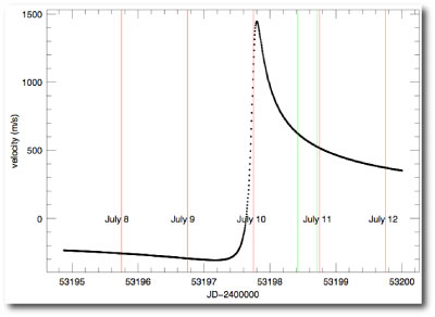
I came down with my first serious case of transit fever (later diagnosed as egressia with complications due to rossiteria) nearly four years ago. The symptoms were brought on by HD 217107, the first candidate planet-bearing star observed by the transitsearch.org network. On the night of August 6th, 2002, photometric data was sent by both an observer in Pleasanton California, and from the KAIT automatic telescope at Lick Observatory. The fits to the radial velocity data indicated that the HD 217107 b transit window was scheduled to begin at 2:40 am PDT, and amazingly, both data sets showed a photometric dip right at the predicted time. To seemingly clinch the case, Debra Fisher also used the Lick 3-meter telescope to obtain five radial velocity measurements of HD217107 during and before the predicted transit ingress. When the spectra were analyzed, the velocities came back with a pattern consistent with the expected Rossiter-McLaughlin effect! [The data is available at this webpage]

To say that I was excited was an understatement. It was my first time out. I had no natural resistance. Tim Castellano, Debra, and I all came down with a full-blown case of transit fever. The period of HD 217107b is 7.127 days, which means that successive transits are spaced one week and 3 hours apart. Tim and I were on the verge of flying with a Meade LX-200 to Hawaii to observe the Aug. 13th transit from the parking lot of the Keck Observatory (That plan, fortunately, was canceled by a combination of high ticket prices and Joe Miller, the cooler-headed then-director of UCO/Lick).

By mid-September, observers in the Canary islands obtained a data set which clearly shows that HD 217107b does not transit. Huge disappointment. At that time, HD 209458 b was still the only known transiting extrasolar planet, and so the second detection would have been a very big deal.

With hindsight, having been innoculated against the transit fever, it’s clear that the transit interpretation was ambiguous in all three of our data sets. For example, in the case of the radial velocities from the Lick 3-meter, a new CCD detector for the spectrograph had just been installed, and so the overall zero point of the velocities relative to the predicted radial velocity curve was a free parameter. If the points are all moved down by 10-15 m/s, then the transit feature turns into ordinary scatter in the data. Likewise, with the photometric data, it was clear in retrospect that systematic effects were at work.

The transit detection problem is tough in part because it’s extraordinarily easy for systematic effects to seemingly conspire to produce an apparent signal. I would not feel confident in announcing a transit until I’ve seen multiple full-transit light curves. On the other hand, though, the false alarms play an important role. They get observers out on the sky, and spur the collection of enough data to truly rule out an event. This certainly wound up being the case for GJ 876, HD 168746, and a number of other candidates.

An early case of transit fever was contracted by U. J. J. LeVerrier, the Nineteenth-century French mathematician famous for the dynamical calculations that led to the prediction and subsequent discovery of Neptune. After the Neptune discovery, LeVerrier turned his attention to explaining the precession of Mercury’s perihelion, and found that the effect could be explained by the presence of a small intra-Mercurial planet that he named Vulcan. After a thorough literature search, LeVerrier unearthed five separate observations of the solar-disk transits by this planet, all at times consistent with predictions. In the following 1877 communication to the Monthly Notices of the Royal Astronomical Society, he’s basically saying, how could all those observations (which agree with theory, no less) possibly be wrong?

As everyone now knows, LeVerrier’s Vulcan doesn’t exist. The 43 extra seconds of Mercurian perihelion precession that had bothered LeVerrier so severely are explained by modifications to classical Newtonian gravity by Einstein’s general theory of relativity.