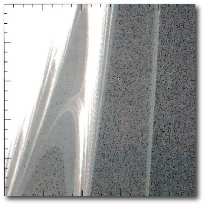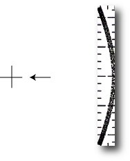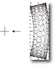
weird orbits in a weird potential

Image Source.

The academic quarter is pulling up to the half-way point at UCSC, and it’s getting tougher to keep up with everything that I’m supposed to do. I’ve been spending a lot of time getting the lectures together, so in the interest of sticking to a schedule of posts, I thought I’d veer from the all-planets-all-the-time approach and show some scanned transparencies from Friday’s class.

The orbit of an idealized planet around an idealized star is a keplerian ellipse. A planet on an elliptical trajectory conserves its eccentricity, orbital period, longitude of periastron, inclination, and line of nodes. The only orbital element that changes over time is the mean anomaly. We can thus say that the Keplerian orbit contains five integrals (constants) of the motion.

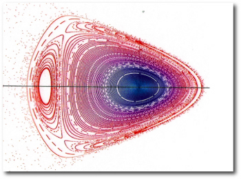
If the potential arises from a mass distribution that’s not a perfect point mass, then in general we won’t have five integrals of motion. It’s interesting to look at a subsection of the weird variety of planar orbits that occur in a two-dimensional potential distribution that looks like this:

The ln(r) term causes this potential goes to negative infinity at the origin while remaining unbounded at large radii. The second term, in which e is specified to take on values between 0 and 1, lends a modulation that makes the force law non-axisymmetric with respect to the origin. One can roughly think of orbits in this potential as the motion of a marble rolling in a funnel-shaped, lopsided bowl.

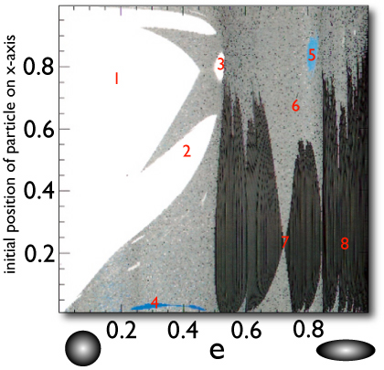
The potential function does not change with time, and so the energy of an orbiting particle is conserved. Further, because of the self-similarity of the potential, the structure of orbits at one energy will be an exact copy of the orbit structures at all other energies. Thus, there’s no loss in generality by sampling orbits having only a single total energy (kinetic + potential). In the following sampler of pictures, I integrate the trajectories of single particles launched from the long (+x) axis of the potential with initial velocities always perpendicular to the long axis. The magnitude of the velocities are determined by the total energy choice: particles starting closer to the origin must have a higher initial kinetic energy to offset their more negative gravitational potential energy. I also vary the parameter e.
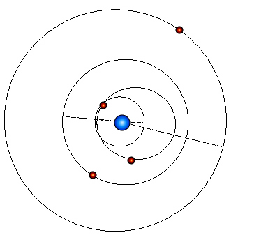
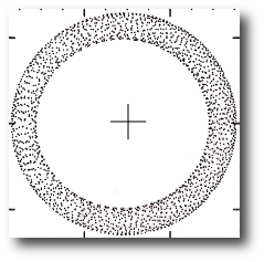
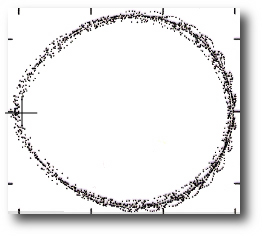
For e=0.2 and an initial position x=0.78, the orbit is reasonably circular, and steady precession smears the excursion of the particle over many orbits into a thin annular region centered on the origin.

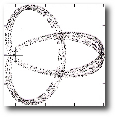
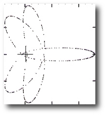
For e=0.42, x=0.55, the particle starts fairly close to its zero velocity curve. It thus falls inward almost to the origin before making a second loop, and then a second approach to the origin which sends it rocketing back up close to its initial position.

Taking e=0.2, x=0.78 leads to a single loop orbit that dives in very close to the origin.

Here’s the result of taking e=0.42 and x=0.55. It’s a good thing the Earth isn’t orbiting in this potential with these particular starting conditions.

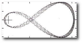
This one, which arises from e=0.81 and x=0.85 is pretty cool. Most of the time it runs counterclockwise as viewed from above, but before close approach to the origin it switches to clockwise. One’s tempted to classify it as an Enron orbit. From all appearances it appears to be clocking a steady increase in angle, whereas in reality, when the books are finally audited, it’s accumulating -2pi radians every period.
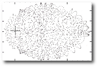
Choosing e-0.30, x=0.03 launches the particle on a highly chaotic trajectory. This orbit is uniformly sampling the entire area allowed to it by its total energy constraint.

For larger values of the e parameter the orbits often show a fundamentally different behavior. Choosing e=0.72, x=0.22 leads to a motion which is restricted to oscillations of a narrow angular range centered on the long-axis of the potential. The particle is basically rolling back and forth in the narrow valley provided by the high-e potential.

e=0.90, x=0.20 gives an orbit with a similar quality:

challenge 4

Image Source.

Eugenio has put the fourth (and final) systemic challenge system on the downloadable systemic console. This dataset is somewhat easier to decipher than the first and second challenges, which were rather esoteric in their planetary configurations. We hope that you’ll find that this one’s a little more down to Earth. I’d like to have your entries in by Oct 31, 23:59 UT. As with our previous three contests, Sky and Telescope is awarding a Star Atlas to the person who achieves the best model of the system.

For this system, it’s likely possible to drive the chi-square arbitrarily close to unity by successively adding spurious, very low-mass planets that act to soak up random noise in the data. We’re currently working on incorporating some standard statistical test utilities into the console which will make it easier to determine whether adding an extra planet is truly necessary. (This will be the topic of an upcoming post, and see the comment thread on Sunday’s post.) For this contest, however, if there are multiple submissions with reduced chi-square near unity, then the prize will be awarded to the fit that also gets the total number of planets in the underlying model correct.

If you haven’t downloaded the console recently, we’re encouraging you to grab a fresh copy. A number of improvements have been added, and there are also a number of additional radial velocity data sets that have been added in recent weeks. Eugenio has been posting a running commentary on the backend describing the console improvements. We’re also putting the final touches on the Systemic Jr. datasets, which we’re hoping to release at the end of next week.

As a result of some articles in the press and on the Internet, we’ve been continuing to see a large increase in the oklo user base. If you’re visiting the site for the first time, you’ll find information about the project and about our goals on the links to the right. Welcome aboard!

1:2:4

Image Source.

The third Systemic Challenge closed to entries on Friday, and I’ve gone through and evaluated the submitted fits. The results were very encouraging. Eight out of twenty-five submissions corresponded to both the correct orbital configuration and the correct number of planets in the underlying dynamical model.

For challenge 003, we looked to our own solar system for inspiration, and tapped the four Gallilean satellites of Jupiter. Eugenio writes:

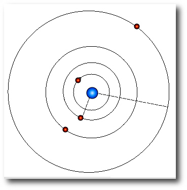
The system is a scaled-up version of Jupiter and the four Galilean satellites. To generate the model, I first set the central mass to 1 solar mass. The (astrocentric) period of Callisto was set to 365.25 days, and I required that the mass and (astrocentric) period ratios in the system would remain the same. Here’s the resulting model (using Jacobi elements, with i~88 deg):

The Challenge 003 System
Parameter “Io” “Europa” “Ganymede” “Callisto”
Period (days) 38.77079 77.77920 156.65300 365.42094
Mass (Jupiters) 0.04926 0.02646 0.08175 0.05936
Mean Anomaly (deg) 99.453 50.772 285.591 47.538
eccentricity 0.003989 0.009792 0.001935 0.007547
omega (deg) 31.229 205.427 303.460 359.879

Among the eight entries that got both the total number of planets and their periods correct, there was a fair amount of variation among fits that had nearly equivalent values for the chi-square statistic. Chuck Smith (among others) turned in a configuration that bears a very strong resemblance to the actual input system. The four planets in his fit all have nearly circular orbits:

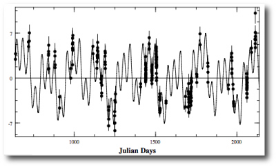
and the resulting radial velocity curve does a very good job of running through the data, with a chi-square value for the integrated fit equal to 1.1005:

A number of other users turned in very similar configurations.

Because of random measurement errors in the data, the true underlying planetary configuration will not necessarily provide the best fit to a given set of radial velocity observations. Often, a better fit can be found for a configuration that is different from the system that generated the data. Steve Undy, for example, achieved a slightly lower chi-square value for his fit by giving a very significant eccentricity to his “Europa”:

The winner of the contest, however, was Eric Diaz, who submitted a 6-planet fit that achieves an integrated chi-square value of 1.04. In addition to the four planets that are actually present in the model, Eric added small planets with periods of 1.06 days and 18.11 days. These objects soaked up some of the residual noise in the fit, allowing for a lower chi-square value, and a copy of the Sky and Telescope star atlas. Nice job Eric!

The contest raises some interesting issues. First, at what point should one stop adding planets to a fit? The chi-square statistic penalizes the inclusion of additional free parameters in a fit, but it’s clear that chi-square can nearly always be lowered by adding additional small bodies to the fit. Second, its very encouraging to see that subtle, but substantially non-interacting systems can be pulled out of radial velocity data sets. In this system, the masses of the planets are small enough so that their dynamical interactions with eachother are not significant over the time-frame that the system is observed. This is in stark contrast to systems such as GJ 876 and 55 Cancri where it is vital to take interactions into account (by fitting with the integrate button clicked on). Finally, I think that we’ll soon see examples of the 1:2:4 Laplace resonance as competitive fits within the existing catalog of radial velocity data sets on the systemic backend.

Gamma Cephei

Image Source.

Guillermo Torres of the CfA recently posted an interesting article on astro-ph in which he takes a detailed look at the planet-bearing binary star system Gamma Cephei.

Gamma Cephei has a long history in the planet-hunting community. In 1988, Campbell, Walker and Yang published radial velocity measurements which show that Gamma Cephei harbors a dim stellar-mass companion with a period of decades. More provocatively, they also noted that the star’s radial velocity curve shows a periodicity consistent with the presence of a Jupiter-mass object in a ~2.5 year orbit around the primary star. In a 1992 paper, however, they adopted a cautious interpretation of their dataset, and argued that the observed variations were likely due to line-profile distortions caused by spots on the stellar surface. From their abstract:

In 1988 Gamma Cep was reported as a single-line, long-period spectroscopic binary with short-term periodic (P = 2.7 yr) residuals which might be caused by a Jupiter-mass companion. Eleven years of data now give a 2.52 yr (K = 27 m/s) period and an indeterminate spectroscopic binary period of not less than 30 yr. While binary motion induced by a Jupiter-mass companion could still explain the periodic residuals, Gamma Cep is almost certainly a velocity variable yellow giant because both the spetrum and (R – I) color indices are typical of luminosity class III. T eff and the trigonometric parallax give 5.8 solar radii independently.

In October 1995, 51 Peg b was announced, and exoplanet research was off to the races. The Walker team, with their futuristic RV surveys had seemingly come close to success, but had not managed to snag the cigar.

In the Fall of 2002, however, the planetary interpretation for the Gamma Cephei radial velocity variations was revived by Hatzes et al., who used McDonald Observatory to extend the data set. They showed that the 2.5 year signal has stayed coherent over two decades, thus effectively ruling out starspots or other stellar activity as the culprit. The planet clearly exists.

Aside from providing a pyrrhic victory for the Walker team, the Gamma Cephei planet is a remarkable discovery in its own right. Its presence showed that gas giants can form in relatively long-period orbits around binary stars of moderate period. In their discovery paper, Hatzes et al. assumed that the binary companion orbits with a period of 57 years, but other estimates varied widely. Walker et al. (1992), for example, adopted 29.9 years, whereas Griffin (2002) use 66 years. The mystery is strengthened by the fact that to date, the companion star has never been seen directly.

The details of the orbit of the binary star are of considerable interest. For configurations where the periastron approach is relatively close, simulations show that the star-planet-star configuration can easily be dynamically unstable.

In his new article, Torres methodically collects all of the available information on the star, and shows that the binary companion to Gamma Cephei has a 66.8 +/- 1.4 year period, an eccentricity of e=0.4085 +/- 0.0065, and a mass of 0.362 +/- 0.022 solar masses. The orbital separation thus lies at the high end of the previous estimates, and renders the stability situation for the system considerably less problematic.

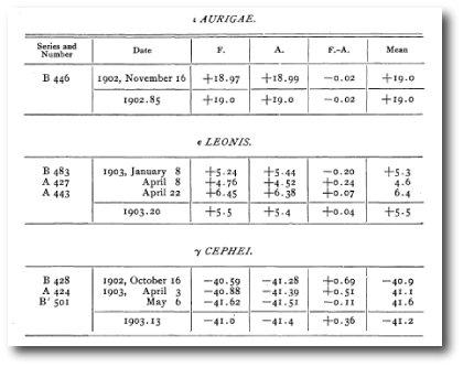
We’re stoked about the Torres paper because it provides references to some truly ancient radial velocities, dating all the way back to a compendium published by Frost and Adams in 1903:

who report 3 measurements made at the University of Chicago’s Yerkes Observatory:

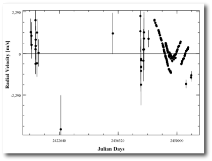
Eugenio has tracked down the various references in the Torres paper, and has recently added all of the available old-school RV’s for Gamma Cephei to the downloadable console. You can access the full dataset by clicking on “GammaCephei_old”:

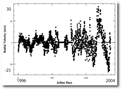
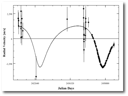
It’s straightforward to manually adjust the offset sliders to put the radial velocities on a rough baseline. You can then build a rough binary star fit with the sliders, followed by repeated clicking on the Levenberg-Marquardt polish button, with the five orbital elements and the five velocity offsets as free parameters. This gives an Msin(i)=386 Jupiter masses, a period of 24,420 days, and an eccentricity, e=0.4112. Try it! The values that you’ll derive are in excellent agreement with the Torres solution:

With the binary fitted out, try zooming in on the more recent data from the past 10-20 years. You’ll see that the modulation of the radial velocity curve arising from the planet is faintly visible even to the eye. It’s interesting to go in and find the best-fit planetary model…

Follow Ups And other items…

Image Source.

It’s very gratifying to see an increasing number of people logging in to the Systemic Backend, and downloading the console. We’ve also been getting a lot of good feedback from users, which we’ll be incorporating into updated versions of the software.

Several people have noted that the backend is currently assigning chi-square values of zero to uploaded fits! We’re highly aware of this problem, and it likely stems from the fact that we may be exceeding our CPU allocation at our ISP. The back-end code integrates all submitted fits to verify the chi-square statistic for purposes of ranking. For submitted systems with long time baselines and short-period planets, these calculations can wind up being fairly expensive. We’ll let you know as soon as this issue gets resolved. In the meantime, it’s fine to submit fits, but if you get a good one, please save a copy in your own fits directory for the time being.

We’ve been getting a lot of entries for the Challenge 003 system. At the end of this week, I’ll tally up the results, so if you’ve got a fit to submit, go ahead and send ‘er in (using the e-mail address listed on the web-page given in the print version of the October Sky and Telescope). It’s fine to submit multiple fits — I’ll use your best one to determine the final ranking. The challenge 003 system represents an interesting dynamical configuration of a type not yet observed for planets in the wild, and so it’ll be very interesting to see what people pull out. Look for Challenge 004 to appear this weekend on the downloadable console, and shortly thereafter, warm up those processors for the advent of the 100 star Systemic Jr. release.

Yesterday’s post is generating an interesting and vigorous discussion thread. Jonathan Langton and I were hopeful yesterday that his benchmark Cassini-State 1 simulation might show an appropriately asymmetric light curve when viewed from lines of sight inclined to the planetary equator (as is the case for the Ups And observations). Frustratingly, however, when the model light curves are actually computed, they wind up drearily sinusoidal, and the phase offset is independant of viewing inclination:

We’re holding out hope, though, for Cassini-State 2. In that case, there are two angles to vary (the orientation of the pole in the orbital plane, and the viewing inclination) and so it may well be possible to dredge up a good fit to the data. After-the-fact parameter tweaking, however, is highly unsatisfactory! I’m looking very much forward to seeing more data sets like Ups And’s. In particular, HD 189733, should give a very nice full-phase curve, and further down the line HD 80606 should be even more interesting.

Darkside

Image Source.

Last week, Joseph Harrington and his collaborators published a paper in Science that announced the results of a very interesting set of observations of Upsilon Andromedae with the Spitzer Space Telescope.

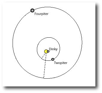
As console users know, Upsilon Andromedae is accompanied by three Jovian planets. The innermost body (officially known as “Dinky“) has at least 70% of Jupiter’s mass and orbits with a period of 4.6 days. Observers have checked to see whether Dinky passes directly in front of the parent star. They found that transits don’t occur, and so the orbital geometry likely looks something like this (as seen from Earth, with the planet grossly not to scale):

Harrington and collaborators made careful measurements of the infrared brightness of the star in the 24-micron band at five known phases during the planetary orbit. These phases are marked with small yellow circles in the above plot.

When the data were reduced, it was found that the brightness of the star was varying in phase with the orbital period of the planet. The brightness is lower when Dinky is in front of the star (near “inferior conjunction”) and higher when more of the planet’s illuminated surface is in view.

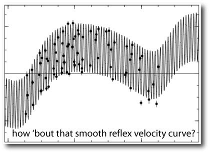
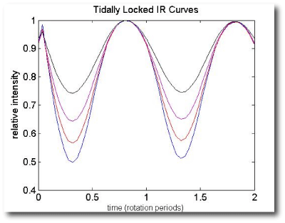
The difference in brightness during the course of the orbit is consistent with a temperature difference of order 1000 K between the illuminated dayside and the dark night side. The planet should be spin-synchronized, so that one side always faces the star and the other face is always pointed away. Harrington et al. showed that the data could be understood if it is assumed that the planet transfers very little heat to the night-side, thus allowing the large temperature difference to be maintained. In fact, they were able to get a good model of the brightness variations by assuming that the night-side was not radiating at all. Such a model curve looks like this:

Intuitively, this result seems to make perfect sense. You’d expect a spin-synchronized planet to be hottest at the subsolar point, and coldest at the antistellar point, and this picture is fully consistent with the five observed fluxes. The results are surprising, however, when we take into account the fact that there should be hellacious winds on the planetary surface which should disgorge heat onto the night side.

UCSC graduate student Jonathan Langton has been studying the surface flows on hot Jupiters using a hydrodynamic technique known as the shallow water approximation. A often-seen feature of his models is that the hottest point on the surface of a synchronously rotating planet is well eastward from the substellar point. (A similar state of affairs is predicted by Cooper and Showman, who use a full 3D GCM-type model.)

Similarly, the coldest spot on the night side, is also displaced eastward from the anti-stellar point:

These models predict a smaller day-night temperature difference than the no-redistribution model that Harrington et al. fitted to the data. A smaller day-night temperature difference can indeed be accomodated by the observations, but the predicted phase shift seems highly inconsistent at first glance. Eastward-displaced hot and cold spots give a (edge-on inclined) lightcurve that is clearly out of phase:

Taken at face value, the observations thus seem to suggest that the flows on the planet are very effective at radiating heat. That is, the upper layers that we can actually observe seem to have a short radiative time constant. In a set of upcoming posts, we’ll have a closer look at the interpretation of this very interesting new result.

TV on the Radio

Image Source.

SETI and the idea of alien life are the stuff of endlessly fascinating speculation. I remember wild late-night conversations with my freshman dorm mates when we should have been writing lab reports and studying for chemistry exams. To date, however, the SETI hasn’t turned up anything, and the Fermi Paradox seems as perplexing as ever. Proponents of the conventional SETI approach argue that this is because we’ve barely scratched the surface in terms of the number of stars that we’ve observed. Build a bigger telescope, they argue, scan more stars, and success will come.

If I look at my own behavior, the trend has been toward increasingly frequent correspondence with more and more people. The cell phone rings many times a day. I send a lot of e-mails via wireless internet. I look on flickr to see if my photos have accumulated views or comments. My life revolves around connectivity. I rarely send letters through regular post, and I have little interest in conversations with a response time of 8.78 years. I’m not inclined to beam coded messages to the sky, and I don’t shine high-power collimated lasers at nearby stars. My behavior is similar in aggregate to many, many others here on Earth.

It seems reasonable, then, that the most promising strategy for a succesful SETI is to look for behaviors that resemble our own. I think it’s much more likely to detect another civilization through their signal “leakage” rather than through reception of a directed message. If I knew that it was going to take at least 8.78, and in all likelihood millions of years for my photos to accumulate views, I’d soon start neglecting to post them.

When I was at the CfA last week, I had an interesting conversation with Avi Loeb, who pointed out that at present, the largest sources of artificial terrestrial radio emission are military radars, FM radio broadcasts, and television broadcasts, all of which emit their power in the frequency range between about 40 and 800 Mhz. SETI searches, on the other hand, have focused in the frequency range above 1 Ghz.

Loeb is involved in the Mileura Wide Field Array (MWA), which is a low-frequency radio telescope designed to study highly redshifted 21 centimeter emission from hydrogen. By mapping the spatial distribution and redshift distribution of 21 centimeter emission, the Mileura project will be able to make a 3-dimensional map of the distribution of atomic hydrogen in the early universe.

The MWA will provide an enormous increase in sensitivity at exactly the frequencies that we here on Earth broadcast. Loeb recently received a grant from the FQXi foundation to run a SETI-search on data obtained during the course of MWA survey observations. The cosmic signals received will be combed for telltale artificial emissions from nearby stars. The array will be sensitive enough to detect Earth-like leakage from more than 1000 of the nearest stars, a list that includes oklo.org Southern Hemisphere favorites such as Alpha Centauri B, Beta Hyi, GJ 780, and Tau Ceti.

Loeb informs me that he’s posted an overview paper on astro-ph. Look for it on Sunday night, 5PM PST.

While we’re on the topic, I recently participated in a panel discussion on SETI that closed up the AIAA Space 2006 meeting in San Jose. I argued that the resolution of the Fermi Paradox lies in the fact that we’re inward bound. My understanding is that the video of the discussion will go up on the web at some point, but for the moment, here’s a .pdf (4MB) file with the transparencies that I showed in my 10 minute summary.

extrasolar trojans

Image Source.

UCSC just put out a press release on the Systemic Project, so if you’re a first-time visitor to oklo.org, welcome aboard. You’ll find information about the project in the list of page links just to the right.

Last week, during my visit to Harvard CfA, I talked to Eric Ford, who has been exploring the idea of searching for trojan companions to extrasolar planets. He pointed out that the discovery of a body in a trojan configuration with a known extrasolar planet would provide an important test of theories of hot Jupiter formation. Here’s a link to his paper.

One way to make a hot Jupiter is to form the planet through the standard core-accretion method at a large radius in the protostellar disk. In this scenario, a newborn gas giant planet starts as a core of rock and ice, which grows to a size of 5-10 Earth masses and begins to rapidly accrete gas from the surrounding nebula. As the planet increases in size, it begins to clear a annular gap in the parent disk. Hydrodynamical simulations (such as the ones reported here, and reproduced in the illustration below) show that L4 and L5, the so-called trojan points located 60 degrees ahead and 60 degrees behind the forming planet, are the last regions of the gap to be cleared out.

It’s possible that co-orbital planets can form from the slow-to-clear material at L4 and L5. When the gas is gone, these objects will remain in stable trojan orbits.

If a pair of planets is caught in a trojan configuration, then they will migrate inward together through the disk, and the migration process will not cause them to become dynamically unstable. Eric points out that the observed presence of a trojan companion to a hot Jupiter would thus be evidence that the hot Jupiter arrived at its short-period orbit via migration. Other possibilities for forming hot Jupiters, such as dynamical instability followed by orbital circularization, do not allow for trojan companions.

A trojan pair of planets presents an interesting conundrum for planet hunters. Normally, a single planet on a circular orbit goes through its radial velocity zero point at the moment when the planet lies on the plane containing the line of sight from the Earth to the parent star. If we have a trojan, however, a planetary transit will be offset from the radial velocity zero point, which is associated with the orbit of a “ghost body” that combines the gravitational effect of the primary planet and its trojan companion. Using the console, try obtaining a two-planet perfect trojan (60 degree separation) fit to a well-known hot Jupiter data set such as that for HD 187123. You’ll find that it’s perfectly possible. The resulting configurations have utterly indistinguishable radial velocity signatures.

Trojans can be detected, however, if the primary planet happens to transit. The presence of the trojan companion can be inferred by measuring the lag between the center of the transit and the zero crossing of the radial velocity curve. For planets with an equal mass ratio, this would amount to a full 1/12 of an orbital period (6 hours for a 3-day orbit).

Which brings up an interesting project for transitsearch.org observers. Most of the known hot Jupiters have been checked photometrically for transits. These transit searches, however, are performed in the time window surrounding the radial velocity zero point. In the (admittedly unlikely) case that some of these objects are trojan pairs with near-equal mass ratios, the transits would have been missed using this approach. To fully rule out transits, one should cover the full 1/6th of an orbital period surrounding the nominal predicted transit time…

stability analysis

Rayleigh Taylor fingers

Image Source.

If you’re spending time on the collaborative systemic backend, you’ll know from the discussion threads that Eugenio has been making rapid progress on the downloadable console. He’s in the process of converting the code from a single-thread version to a fully multi-threaded package. Threading is important. It will allow the console to be gracefully reset in the event that a Levenberg-Marquardt polish takes more time than you bargained for, and it will allow for a variety of on-the-fly diagnostics regarding what’s going on under the hood.

The latest version of the downloadable console now contains a multi-threaded orbital stability checker. To see it in action, download a fresh console (making sure to save your old systemic directory if you have built up a library of fits that you want to keep). I pulled up the HD 69830 dataset and quickly worked up a three-Neptune fit that is very similar to the fit reported by the Geneva team in their discovery paper.

The two outer planets are roughly similar in mass to Neptune, while the inner planet, with a period of 8.66 days is somewhat less massive. It’s not immediately clear from looking at the orbital configuration:

that this planetary troika is gonna get along to go along. A stability check is definitely in order. Clicking on the button for the long-term stability module:

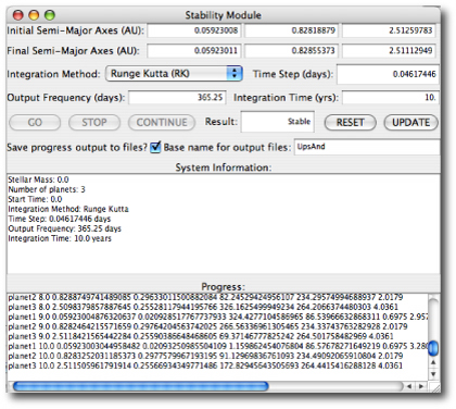
brings up a dialog window that you can use to control the stability integration. You specify the maximum timestep duration, the output frequency, and the integration duration and press go. At present, the console implements only a 4th/5th order Runge-Kutta integrator, but we’ll soon supply faster algorithms, including a Wisdom-Holman symplectic map:

For this example, I specified a short 100-year integration (4200 inner planet orbits). This is enough to see whether the system is wildly unstable, but for a more diagnostic check, one would generally like to look at a longer duration (100,000 inner planet orbits, say).

In this first implementation, a system is deemed “stable” if the semi-major axes of all the planets remain constant to within 1% of their initial values during the course of the integration. There are, of course, stable systems (such as a librating, equal-mass 1:1 resonance configuration) where larger semi-axis variations occur, but if semi-major axes vary by more than 1%, it means that considerable orbital energy is being traded back and forth, and the long-term prognosis is not good.

This HD 69830 3-planet fit easily lasts for 100 years. Nevertheless, as noted in the discovery paper, longer-term integrations show that the system is very close to the edge of stability.

I’m still working on the promised post about trojan planets. Look for it tomorrow!

And inside the second envelope…

Image Source.

First, a thank-you to everyone who submitted a fit to the second systemic challenge. I just loaded all the fits into the console and evaluated the chi-squares (with integration turned on). Jose Fernandes, of Lisbon, Portugal, submitted the winner, and will be receiving the $149.99 sky atlas from Sky and Telescope.

Jose’s fit has a reduced chi-square statistic of 3.94, and is comprised of three planets:

The outer two bodies have masses 1.58 and 0.5 times that of Jupiter, with eccentricities of 0.58 and 0.14. They share a common period of 362 days. The fit also has a tiny inner planet with a mass just under 3% that of Jupiter and a period of 50 days. This little guy improves the fit by wriggling the radial velocity curve up and down to statistically grab more points.

The system that actually generated the data was quite similar:

There are two equal-mass planets with masses 1.04 times that of Jupiter, with eccentricities of 0.7 and 0.2. They share a common period of 365 days. The 50-day planet in the winning fit was spurious, as is often the case when a model planet has a mass that is far smaller than its companions.

This system is an example of a one-to-one eccentric resonance. It is based on a system that was discovered by UCSC physics student Albert Briseno in one of the simulations that he ran for his undergraduate thesis, and it was formed as the result of an instability in a system that originally contained more planets. The system experienced a severe dynamical interaction, which led to a series of ejections. After the last ejection, two planets remained. They share a common orbital period, and gradually trade their eccentricity back and forth. Their interaction gives a strong non-Keplerian component to the resulting radial velocity curve for the star, which makes this a tricky system to fit. While the system might seem absurdly exotic, it’s recently been suggested by Gozdziewski and Konacki that HD 82943 and HD 128311 might have their planets in this configuration (you can of course try investigating this hypothesis for yourself with the console). Their paper is here.

The challenge 002 system is an example of a general class of co-orbital configurations in which the two bodies constitute a retrograde double planet. If you stand on the surface of either world, the other planet appears to be making a slow retrograde orbit around your moving vantage as the libration cycle unfolds over several hundred orbits.

In tomorrow’s post, we’ll stay on the topic of co-orbital planets, and look at some interesting new work by Eric Ford on the possibility that we might soon be able to observe planets in Trojan configurations. Two planets in a Trojan orbit librate around the points of an equilateral triangle in the rotating frame. Indeed, when such an arrangement occurs, it’s possible that a particularly interesting dataset might have the capacity to launch a thousand fits.

[For more about 1:1 resonances, see this post and this post. For a discussion about the audio wave forms that they produce, see this post.]

CfA

Image Source.

Back from a great visit to the Harvard CfA. The exoplanet research effort out there is amazingly comprehensive, and I soaked up a whole range of interesting news items to report. A slew of posts are in the works.

I’ve uploaded my colloquium talk in (1) Apple Keynote format (harvard.key.tar.gz) , (2) Powerpoint format (harvard.ppt.tar.gz), and (3) as a set of .pdfs. The talk was built in Keynote, and thus will look best in that format. Note that the Keynote and Powerpoint files are both quite large (~58MB compressed, ~90MB uncompressed) because they contain a variety of animations. The .pdfs amount to about 7 MB, and show only the splash frames from the animations. Feel free to use any of these slides in presentations or classes (with a shout-out to oklo.org).


Eugenio has been working hard on the console during the past few days. The downloadable version now contains a stability checker which integrates a fit for a user-specified period. Relative changes in the semi-major axes of more than 1% are then used to flag instability. Give it a whirl! We’ll discuss it in more detail in an upcoming post.

Tomorrow, I’ll announce the results of the second systemic challenge. The third challenge system is already available on the downloadable console.

Some updates

Image Source.

I’ll be gone on a trip to the Harvard CfA for the next several days. While I’m there, I’ll be giving a colloquium talk, and in addition, I’ll be trying to extract all the latest research news items from the CfA’s large group of exoplanet researchers. That’ll likely give me some stuff to write about in upcoming posts.

We’ve now closed the Systemic Challenge 002 contest, and I’ll tally up the results on the plane ride home. Look for a post this weekend that will explain what’s going on in the Challenge 002 data set. Eugenio has cooked up a great batch of RVs for the Challenge 003 system, and we’ll be releasing them this coming weekend.

Note that the dates of the challenges are slipping from what was announced in the S&T article. There’ll still be a total of four systems, but the contests will run over two months rather than one as originally planned. As soon as the contests are finished up, we’ll release the “Systemic Jr.” set of 100 trial systems. Based on our experience with these systems, we’ll make any necessary modifications to the simulation profile, and then we’ll be set to start the long-promised full Systemic simulation. In the meantime, keep submitting fits! I’d really like to see the chi-square come down on a dynamically stable configuration for 55 Cancri.

In other news, we’ve now got confirmations for both WASP-1b and WASP-2b.

On Monday, Mike Fleenor, of Volunteer Observatory in Knoxville Tennessee wrote:

I observed a complete transit of WASP-1b last night under very good conditions. My LC shows mid-transit very close to your predicted center. Details are available here.

Last weekend, Joe Garlitz from Elgin Oregon wrote:

Last night (Fri/Sat) I tried for WASP2 and got some data that looks promising. The data is very noisy and I would not feel comfortable about presenting it without some other confirming (hopefully someone else got data) observations.

I have attached a .jpg image of the data chart. The data is really forced to get any kind of “curve”. The solid line represents a running average over 16.25 minutes, 13 data points.

The individual images are 65sec at an interval of 75 sec. The scope is 200mm @ f/8 with a Cookbook 245 CCD, no filters.

Here’s his lightcurve:

Today, Geir Klingenberg from Norway checked in with a confirmation of Garlitz’s result (which he obtained remotely from a telescope in New Mexico:

Hi Joe,

I observed the ingress of this WASP-2 transit, see here.

Seems to fit your data nicely.

I used a robotic telescope at GRAS: 0.3m SCT @ f/11.9 and a FLI IMG1024.

Way to go, guys!

speculations

Image Source.

Hey Everybody, if you’ve been working on your fits to the second Systemic challenge system, send them to the e-mail address listed on the web-page given in the Sky and Telescope article.

I’ve been hearing many rumors floating around that there’s going to be a big planet announcement next week. Unfortunately, oklo.org has not yet joined the privileged ranks of the mainstream science press, so I haven’t been privy to any advance looks at the result that’s gonna come off the wire. I did hear, though, that it’s going to be an STScI announcement, so I did a little anticipatory detective work.

STScI runs HST, which means that the result will be the product of Hubble observations. In order to make Hubble observations, one needs to manage to get a block of fiercely competitive Hubble time, which means you need to write a successful Hubble proposal. The abstracts of winning Hubble proposals are posted publicly on NASA ADS. A quick search yields the following accepted proposal abstract (Proposal ID #10466), submitted by Dr. K. C. Sahu:

We propose to observe a Galactic bulge field continuously with ACS/WFC over a 7-day period. We will monitor ~167, 000 F, G, and K dwarfs down to V=23, in order to detect transits by orbiting Jovian planets. If the frequency of “hot Jupiters” is similar to that in the solar neighborhood, we will detect over 100 planets, more than doubling the number of extrasolar planets known. For the brighter stars with transits, we will confirm the planetary nature of the companions through radial- velocity measurements using the 8-m VLT. We will determine the metallicities of most of the planet-bearing stars as well as a control sample, through follow-up VLT spectroscopy. The metallicities of the target stars range over more than 1.5 dex, allowing for a determination of the dependence of planet frequency upon metallicity–a crucial element in understanding planet formation. We will be able to discriminate between the equally numerous disk and bulge stars via proper motions. Hence we will determine, for the first time, the frequencies of planets in two entirely different stellar populations. We will also determine for the first time the distribution of planetary radii for extrasolar planets for both these populations. Parallel observations with NICMOS will provide ultra-deep near-infrared images of a nearby bulge field, which will be used to determine the stellar luminosity and mass functions down to the brown-dwarf regime. The data will also be useful for a variety of spinoff projects, including a census of variable stars and of hot white dwarfs in the bulge, and the metallicity distribution of bulge dwarfs.

I looked at Sahu’s web page at STScI, where he writes:

At present, my research is mainly focused on a large HST program which involves monitoring of about 300,000 stars towards the Galactic bulge using the Advanced Camera System (ACS) on board HST, to search for extra-solar planets. The results are due to appear in the October 5, 2006 issue of Nature.

So clearly, the ACS data have been reduced, and it’s an excellent bet that they’re planning to announce the transit candidates that have emerged from their 7 days worth of ACS photometry. The number of transits to be announced is almost certainly more than two. This week’s announcement of WASP-1b and WASP-2b certainly didn’t produce a noticeable media splash, so there must be a lot of planets in the announcement. And given the past history of HST microlensing planet detections, I bet it’ll be the case that some of the parent stars of the soon-to-be-announced new transiting planets have indeed undergone a fairly rigorous spectroscopic follow-up with the VLT.

I think that spending a whole week of ACS time to stare at stars in the galactic bulge is a fairly worthwhile use of the HST (although I bet a lot of extragalactic astronomers might disagree). Here’s my take: In the mid-1990’s, it was believed that the stars of the galactic bulge are very metal-rich. In 1994, for example, McWillian and Rich 1994 reported an average bulge star metallicity of 0.2 “dex”, that is, ~60% greater than the solar value. More recently, however, Fulbright et al. 2006 have revised the average metallicity of the bulge downward to a value of -0.1 dex (~80% of the solar value). It thus appears that the metallicity distribution of the stars in the bulge is roughly similar to the metallicity distribution of stars in the solar neighborhood.

We know from Debra Fischer and Jeff Valenti’s work that the rate of short-period giant planet occurence is a strong function of stellar metallicity:

the planet metallicity correlation

All other things being equal, we can use the above diagram to inform an estimate of the number of planets that Sahu and company will announce. The hot Jupiter occurence rate in a solar-neighborhood type metallicity population is of order 0.7%. About 10% of hot Jupiters will be observable in transit. About half of those transits will be clobbered by the effect of a binary companion sharing the pixel and driving the detection below threshold. For a 7-day survey, about 60% of the hot Jupiters will actually get picked up, given constant coverage and good control of detector systematics (which HST certainly has). This means that Sahu should see (167,000)x(0.007)x(0.1)x(0.5)x(0.6)=35 transiting planets.

The problem, however, will be that there are many events which will look like planet transits, including grazing eclipsing binary stars, transiting M-dwarf stars, and the surprisingly common situation where a background eclipsing binary star shares the pixel with a foreground target star, a so-called blend situation. Dave Charbonneau and his collaborators have written extensively about all of the different pitfalls that can cause a wide-field transit survey to turn up false positives.

So my guess is that there will be of order 200 transit candidates in the ACS data for 167,000 stars. The brightest and most promising of these will have been sent to the VLT for spectroscopic follow-up. If the sensitivity limit of the survey (as stated in the proposal abstract) is V~23, then the candidate stars will likely have V~20-21. Even with the VLT, it’s tough to get accurate radial velocity measurements for stars this dim. So a lack of an observed binary stellar companion will probably be taken as a confirmation of the presence of a planet. (This is all complete speculation on my part.) Going even further out on a limb, my guess is that they have ~100 stars that show transit signatures, and which do not have a spectroscopically detectable binary stellar companion. Although it’ll be hard to further sort the wheat from the chaff, I’ll harbor a guess that 1/3 of the planets that will likely be announced are bona-fide.

Assuming that this is what actually occurs at the press conference, then we’ll have a very interesting result — not so much about the planets (which will be hard to characterize owing to the dim parent stars) — but because of what it tells us about the formation of the galactic bulge. Right now, there are several competing theories for how the bulge formed. One possibility is that scattering of stars by the Milky Way’s galactic bar has populated the Milky Way’s bulge with stars. Another possibility is that the bulge stars are the result of many disrupted globlular cluster or dwarf-galaxy like objects.

A measurement of the planet population of the bulge stars can allow us to distinguish between these two possiblities. If the planet occurance rate is similar to the galactic neighborhood (which I’m guessing will be the gist of the press conference) then the bulge stars are likely to have formed under low-density conditions. This would favor a bar-scattering type of scenario. If the planet occurence rate is zero or very low (which is unlikely, given that they are having a press conference) that would imply that the stars formed in a high-density environment. A crowded star formation leads to a ultraviolet ionizing radiation field that makes it difficult for planets to form and then migrate inward to become hot Jupiters.

There was a remarkable study done with HST in the late 1990s, and published by Gilliland et al. 2000. HST obtained a 8.3-day photometric time series for 34,000 stars in the globular cluster 47 Tucanae. The data, when reduced, show a total absence of transiting planets. This result shows the power of both the environment variable (the 47 Tucanae stars formed in an intensely irradiated region of star formation) and the metallicity variable (the metallicity of the 47 Tucanae stars is about 20% the solar value).

Finally, it’s always good to look at costs. According to the Wikipedia, the total cost of building, launching, servicing, and running HST has been of order 6 billion dollars. It started working as planned in 1994, and will thus have ~15 years of fully functional use. The seven days of ACS time were therefore worth 7.6 million dollars. This is comfortably more than the cost of building a special-purpose telescope to probe the terrestrial planets that are almost certainly orbiting Alpha Centauri B. (For more information, see these oklo.org posts: 1, 2, 3, 4, 5.)

HJD

These thumbnails show 42 of 56 photos taken during the interval from 6:56:27 PM to 7:00:26 PM CDT on September 16th, 2006, at spacing of roughly 3.2 seconds per frame. We were northbound on Interstate 57, north of Tuscola, Illinois.

I’ve processed the frames into animations, which can be accessed in mov and mp4 formats: tuscola.mov (200 kB) and tuscola.mp4 (600 kB). There’s an interesting sense of high-speed motion imparted by the differential blur and the decreasing altitude of the Sun above the horizon. I used a zoom factor of 10x, and was aided by the extremely level landscape. It was very flat because we were just north of the maximum southern extent of the Wisconsinan glaciation, which retreated just 13,000 years ago.

The animation demonstrates that just south of 40 degrees north latitude, the duration of Sunset near the equinox is just under three minutes. As I watched the Sun go down, I was thinking about the fact that the Earth’s motion through its orbit is creating transits observable (in September) to observers located on planets orbiting specific stars lying in Pisces.

Here on Earth, observations of transiting extrasolar planets are mediated by a complex beat pattern between the diurnal and seasonal cycles of the Earth, and the alien periodicity of the transiting planet. Assuming clear weather, in order to catch a complete predicted transit it needs to be dark, and at least a transit duration before dawn. In addition, the target star needs to maintain a sufficient altitude above the horizon during the course of the transit.

These constraints have restricted the aggregate of known transits to objects with periods of 4 days or less. From a single location on Earth, it’s very hard to find and confirm transiting planets with longer periods. With a global network, however, the problem is more manageable, essentially because it’s always 5pm somewhere. Several years ago, we published a detailed analysis which shows quantitatively how a network of small telescopes gains in advantage over a single large telescope at a fixed location as the planetary period increases.

and then there were fourteen…

In June 2002, I saw Keith Horne give a review talk at the Scientific Frontiers in Research on Extrasolar Planets Meeting at the Carnegie Institute of Washington. He showed a slide (an updated version of which is here) that listed 23 planetary transit surveys that were in operation at that time. He had asked the investigators running each survey to send him the number of new transiting planets per month that could be expected to turn up. The grand total rang up to a whopping 191 fresh planets per month, or 2,292 planets per year.

For a number of reasons, those numbers haven’t quite panned out, but it nevertheless finally looks like we’re entering a phase where the planetary yield from wide-field transit surveys is starting to ramp up dramatically. Today’s astro-ph mailing has a paper by Collier Cameron et al. entitled “WASP-1b and WASP-2b: Two new transiting exoplanets detected with SuperWASP and SOPHIE”, describing the discovery of P=2.15 d and P=2.52 d planets transiting ~12th magnitude stars. As of this month, astronomers have been hauling in transits at a rate of one per week.

Dave Charbonneau at CfA dropped me an e-mail this morning:

Great chance to catch WASP-1 tonight from the western US. We will pursue it from Mt. Hopkins and Palomar, but thought you might want to give a heads up to transitsearch.org. This one is very much in need of a great light curve, as the current estimates of the planetary radius range from “smallish” to “huge”, with an error bar that is depressingly large.

He’s definitely right about all that. Multiple photometric data sets will be of considerable use in constraining the system parameters. It’s also going to be very important to get a better handle on the properties (Mass, Radius, and metallicity) of the WASP-1b and 2b parent stars. We’d really like to know how these two new planets fit into the overall trends that are starting to emerge among the aggregate of transiting planets.

Ephemerides for both of the WASPs have been added to the transitsearch.org candidates table, and the (rather meagre) published tables of radial velocity measurements have been added to the Systemic back-end. Given the short orbital periods, I don’t think it’ll be very long at all before small telescope observers start producing confirmation light curves.