Armchair Planet Hunting

Image Source.

The Associated Press just published an article on how the Internet has facilitated an increasing number of collaborations between amateur and professional astronomers. The systemic project is one focus of the AP piece, and we’re seeing a jump in traffic as a result. If you are a first-time visitor to the site, welcome aboard!

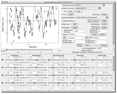
There are several ways that you can use and participate in systemic. Our project home page is a weblog (updated fairly frequently) that gives an insider’s perspective on the latest developments and discoveries in the fast-moving fields of extrasolar planets and solar-system exploration. We write for a target audience of non-astronomers who are interested in astronomy. To get a flavor for the blog, keep reading the posts below, or have a look at a few of our past articles, such as our take on last Summer’s big “is Pluto a planet debate”, our exploration of what planets and galaxies really look like, or our series [1, 2, 3, 4] on the feasibility of detecting habitable terrestrial planets in the Alpha Centauri System.

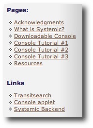
You should see a set of links just to your right:

These links give you information that you can use to start participating in the actual discovery and characterization of extrasolar planets. (Despite the fact that we’re rocket scientists, we’ve been unable to consistently sweet-talk Microsoft IE into correctly displaying our site. On some versions of IE, you may have to scroll all the way down to the bottom of this page to see the links). The Downloadable Systemic Console is our Java-based software package that allows you to work with extrasolar planet data. The Systemic Backend is a collaborative environment that has the look and functionality of a social networking site. Registration and participation are free. The nearest well-characterized extrasolar planets (GJ 876 b, c and d) are 14.65 light years away, and so the news of useful modern innovations such as pop-ups and spyware hasn’t had time to propagate to those far-distant worlds. Hence the systemic backend is completely free of annoying ads!

One final note: there are two separate channels for registration on systemic. The first, accessed through the “login” tab on the site header above, is part of the WordPress package that runs the blog. Registration on the blog allows you to comment on our frontend posts. The second, accessed through the “backend” tab on the site header or the link to the right, gives you access to the collaborative php-based environment that constitutes the systemic backend. You can register for either or both, and you don’t need to give your real name or any real-world identifying information other than an e-mail address.

Tune in regularly for more news and updates.

So Which Planet is on Your Coffee Table?


Image Source.

Newly published high-profile books get set out prominently on the display tables at the front of Borders in downtown Santa Cruz. During this past holiday season, one of the prime spots was given to Postcards from Mars by Cornell’s Jim Bell, who is the Pancam lead scientist for NASA’s Mars Exploration Rover Mission. The book is superbly produced. The Pancams’ high resolution allows the photos in the fold-out spreads to convey an impact that’s hard to achieve by surfing the NASA website with your browser.

With all the focus on Mars, I think the public tends to forget that Cassini, NASA’s flagship mission, is sending back an even more amazing trove of images from a far more alien environment. Indeed, Jeff Cuzzi (a colleague from my NASA Ames days) along with Laura Lovett and Joan Horvath, have just written a coffee-table book, Saturn A New View, that highlights the most stunning images of the Saturnian system. At the moment, the book is buried back in the science section at Borders, but it absolutely deserves a spot out in front as well. The “upgrade”, if you will, from Voyager to Cassini is an order of magnitude more impressive than the jump from Viking to Spirit and Opportunity.

I was nine years old when Viking 1 landed on Mars in 1976, and I vividly remember seeing the first images of the martian surface on the CBS morning news. I also recall that I was quite interested when the Voyagers sent back the first close-ups of Saturn and its environs, but I can’t remember the exact moment of seeing those photos for the first time. A quarter century later, this same gap in enthusiasm is reflected by the fact that the Mars book has an Amazon sales rank that is way ahead of the Saturn book.

On Mars, when you look at the landscape, the scene is familiar. It looks like a rocky desert on Earth. In the mind’s eye, you can place yourself on the surface. You can imagine hiking into the hills on the horizon. In short, you know what you’re seeing.

Image Source.

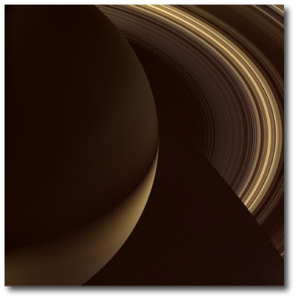
With Saturn, on the other hand, the views are abstract and alien. We don’t have rings in our sky, and so I’m intuitively unfamiliar with the play of shadows on the surface of the planet and the rings. When you look at views of Saturn, there’s no sense of being “right there”. You have to think more carefully to really see what you are seeing.

Image Source.

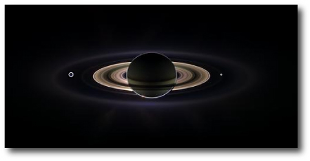
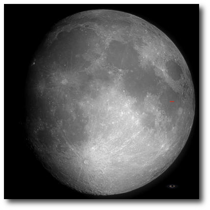
It amazes me that the size of Saturn and its rings is quite comparable to the Earth-Moon distance. Using Illustrator to superimpose the Earth and the Moon on the Saturnian system, the scale looks like this:

It took the Apollo astronauts about a day to traverse a distance equivalent to the diameter of Saturn. (It took them three days to make the trip from the Earth to the Moon.)

From Earth, when Saturn is visible overhead at midnight, it lies about 8.5 AU away. This means that the diameter of the A-ring subtends about 3/4 of an arc minute in the sky. That’s somewhat below the resolution limit of the human eye. If Saturn lay at Jupiter’s distance, however, people with sharp eyes would just barely be able to distinguish it as appearing slightly oblong.

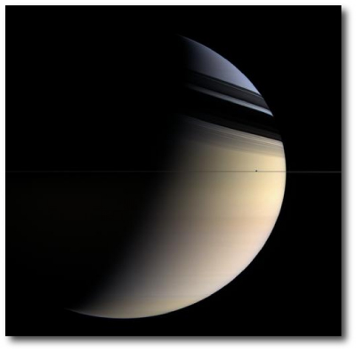
Until I read the new Saturn book, I had not realized that the northern hemisphere of Saturn currently appears blue. It’s winter in Saturn’s northern hemisphere, and the tilt of the rings blocks additional sunlight from reaching the upper half of the planet. The frigid conditions have caused the ochre-colored haze to dissipate, and we have a view down to the methane-rich red-absorbing regions at greater depth. It’s the same effect that gives Neptune and Uranus their blue cast.

Billions of years from now, after the Sun has turned into a white dwarf, and after the planets have lost the majority of their internal heat, all four giant planets will take on the blueish color that Neptune and Uranus currently have. The current color of Saturn’s frigid northern hemisphere is an early preview of things to come.

Happy New Anomalistic Year

Image Source.

Jan 1st, the first day of the year in the Gregorian civil calendar, is an artificial construction with no actual physical significance. The real new year started yesterday, Jan 3rd, at 20h UT, when Earth passed through perihelion (the point where its orbit is closest to the Sun).

As a result of planet-planet perturbations, the apsidal line of Earth’s orbit precesses with a period of 21,000 years. The anomalistic year (the time between periastron passages) is thus about 25 minutes longer than the familiar tropical year, which means that everyone is allowed to show up 25 minutes late for work this week.

Even when precession is considered, Earth’s orbit exhibits quite a nice clockwork regularity. This is in considerable contrast to the outer planets “b” and “c” in the GJ 876 system, where the anomalistic year is truly anomalistic. The resonant interactions between the planets cause successive inferior conjunctions to vary in a complicated manner by more than 4 hours to either side of the average period.

The Earth’s year could get completely deranged if another star (or multiple star) in the local galactic neighborhood makes a close approach to the solar system. Back in the late 1990’s, Fred Adams and I took a close look at the odds that the solar system will get disrupted by such an encounter before the Sun turns into a red giant. We did a large set of Monte-Carlo scattering calculations, and found that there’s about a 1 in 200,000 chance that the Earth will find its orbit seriously disrupted before the Sun drives a runaway greenhouse effect on the Earth’s surface. There’s also about a 1 in 2,000,000 chance that the Earth will get captured into orbit by another star before the Sun destroys the biosphere. If this galavanting incoming star turns out to be a red dwarf, then we’ll be set for a trillion-plus years of steady luminosity. One in two million sounds like a very low probability, but people regularly line up to buy powerball tickets with far less chance of striking the jackpot. After all, someone’s gotta win.

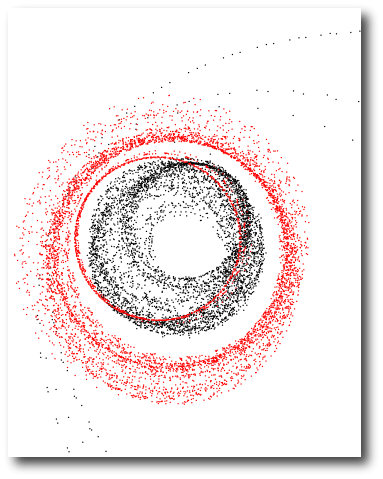
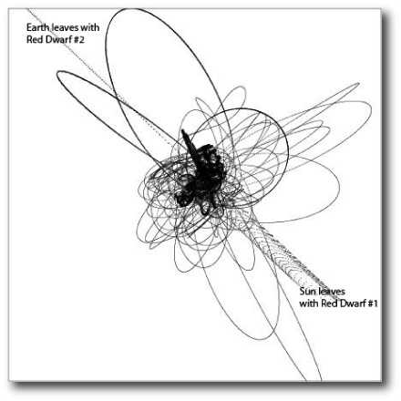
Here’s an example of a specific capture scenario:

In the above picture, a red dwarf binary pair makes a close approach to the solar system from the direction perpendicular to the screen. As the red dwarfs drop toward the Sun, Earth is almost immediately handed off to the smaller dwarf and stays with that star for three long, looping excursions. After slightly more than 1000 years, Earth is palmed back off onto the Sun, with whom it remains for the next 6500 years while suffering many complicated close encounters with the other stars. After 7500 years, Earth is captured into an orbit around the larger red dwarf, and soon thereafter, this star escapes. Earth is pulled along in an elliptical orbit that might possibly be habitable.

For more on the bizarre panoply of events that might occur in the distant future, check out my book with Fred Adams: The Five Ages of the Universe — Inside the Physics of Eternity. Its long-term view can provide a certain antidote to an overscheduled workweek…

[On the topic of red dwarfs, an upcoming oklo post will be by Systemic team member Paul Shankland, who’ll be reporting in on the survey he’s leading to find habitable planets transiting low-mass nearby stars.]

Roll ’em out…

Image Source.

The discovery of new planets is rarely clear cut. No sooner does a new world (Vesta, Neptune, Pluto) emerge, than the wrangling for the credit or the naming rights starts. And it’s usually possible to find a reason why the prediction (or even the planet itself) wasn’t really valid in the first place.

The trans-Uranian planet predicted by Urbain J. J. Le Verrier and John Couch Adams happened to coincide quite closely with Neptune’s actual sky position in September 1846, but the orbital periods of their models were too long by more than 50 years. Le Verrier’s predicted planetary mass, furthermore, was too large by nearly a factor of three, and Adams’ mass prediction was off by close to a factor of two.

In England, following the announcement of Neptune’s discovery, and with the glory flowing to Le Verrier in particular and France in general, the Rev. James Challis and the Astronomer Royal George Airy were denounced for not doing enough to follow up Adams’ predictions, “Oh! curse their narcotic Souls!” wrote Adam Sedgwick, professor of geology at Trinity College.

Nowadays, with the planet count up over 200, the prediction and discovery of a new world doesn’t quite carry the same freight as it did in 1846. No editorial cartoons, no Orders of Empire, and no extravagant public praise to the discoverer, such as that heaped by Camille Flammarion on Le Verrrier, who wrote, “This scientist, this genius, has discovered a star with the tip of his pen, without other instrument than the strength of his calculations alone!”

Nevertheless, I don’t want to be shoehorned into the ranks of the “narcotic souls” as a result of not properly encouraging the bringing to light of any potential planetary discoveries in the systemic catalog of real stellar radial velocity data sets. As of Dec. 30th, 2006, over 3,680 orbital fits have been uploaded to the systemic backend. It’s definitely time to start sifting carefully through the results that the 518 registered systemic users have produced. Over the next few weeks we’ll be introducing a variety of analysis and cataloging tools that will make this job easier, but there are some interesting questions that can be answered right away. Foremost among these is: what are the most credible (previously unannounced) planets in the database?

The backend uses the so-called reduced chi-square statistic as a convenient metric for rank-ordering fits:

In the above expression, N is the number of radial velocity data points, and M is the number of activated fitting parameters. As a rule of thumb, a reduced chi-square value near unity is indicative of a “good” fit to the data, but this rule is not exact, and should hence be applied with caution. The observational errors likely depart from a normal distribution, and more importantly, the tabulated errors don’t incorporate the astrophysical radial velocity noise produced by activity on the parent star. Furthermore, it’s almost always possible to lower the reduced chi-square statistic by introducing an extra low-mass planet.

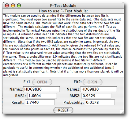
Eugenio recently implemented the downloadable console‘s F-test, which can provide help in evaluating whether an additional planet is warranted. The F-test is applied to two saved fits and returns a probability that the two fits are statistically identical. As an example, pull up the HD 69830 data set and obtain the best two planet fit that includes the 8.666-planets and 31-day planets. Save this fit to disk. Next, add the 200-day outer planet and save the resulting 3-planet fit to disk (using a separate name). Clicking on the console’s F-test button allows the F-test to be computed using the two saved fits:

In the case of HD 69830, there’s a 1.7% probability that the 2-planet fit and the 3-planet fit are statistically identical. This low probability indicates that the third planet is providing a significant improvement to the characterization of the data. It’s likely really out there orbiting the star.

So here’s the plan: Let’s comb through the systemic “Real Star” catalog, and find the systems that (1) contain an unannounced planet(s) in addition to the previously announced members of the system (see the exoplanet.eu catalog for the up-to-date list). (2) have a F-test probability of less than 2% of being statistically identical, and (3) are dynamically stable for at least 10,000 years. If you find a system that meets these requirements, post your findings to the comments section of this post.

Disclaimer: this exercise is for the satisfaction of obtaining a better understanding of the planetary census, and also for fun. When the planets do turn up, I’m going to sit back with a bottle full of bub and enjoy any scrambles for priority from a safe distance.

Happy New Year, y’all!

A World-Encircled Sea

Image Source.

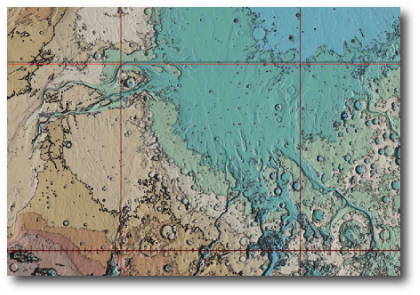
I now have a topographic Mars globe on my desk, and I’ve been staring at it. It’s common knowledge that the northern Martian hemisphere is low-lying and nearly uncratered, but this was never hammered home to me until I spent time staring at an actual globe, tracing the shorelines of the vanished ocean.

Image Source.

The Mass-Period Diagram

radio -- live transmission

Image Source.

When J. Edgar Hoover was getting on in years, his aides would often tell scheduled visitors to his office that he was unable to meet with them because he was “in conference”. In reality, this meant that Hoover was napping at his desk.

It might seem that the refrain of, “we’re busy working on the systemic back-end” is an equally convenient euphemism for long lapses between posts on the front end. Nevertheless, we have been busy getting the new oklo xserve quad xeon up and running. The whole site has now been replicated and tested, the server is live and on air, and very shortly, we’ll be flipping the switch. Can’t wait, man!

With the vast increase in processing power afforded by the xserve, we’ll be able to provide a much more extensive suite of research tools to oklo visitors. In particular, it’ll be possible to dynamically generate the kinds of correlation diagrams that are currently only available from our estimable continental competition: exoplanet.eu.

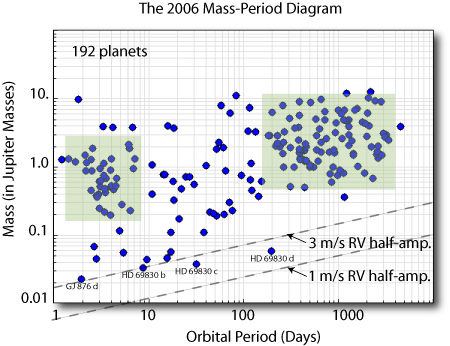
It’s always interesting to look through the latest versions of the correlation diagrams to see whether the various trends and hints of trends are holding up. The a-e plot is worth examining, as is the plot that charts the number of planetary discoveries per year over the past decade. As of today, exoplanet.eu lists 192 planets that have been detected with the radial velocity method. Plotting the masses of these planets against their periods on a log-log plot (and running the resulting screenshot through Illustrator) yields the following:

latest mass-period diagram

For Keplerian orbits, the relationship between the radial velocity half-amplitude of the parent star and the orbital period of the planet is given by:

equation for radial velocity half-amplitude

If we assume that the mass of the planet is negligible in comparison to the mass of the star and if we further assume edge-on, circular orbits around solar mass stars, then we get the dashed lines in the figure that show detection thresholds for K=3 m/s and K=1 m/s. The three planets orbiting HD 69830 stand out in this diagram as the most striking discoveries of 2006.

To the eye, there are two curious clusters of planets in the diagram. At short periods (P~3d) we have the hot Jupiters. Most of these have masses (times the sine of the unknown inclination) somewhat less than Jupiter. At longer periods (P>100d) we have a second prominent clump of planets. These are the Eccentric Giants, and their masses average out at a significantly higher value (between 2 and 3 times the mass of Jupiter). Part of the difference in mass is due to selection bias, but nevertheless there is a real effect. Like the planet-metallicity connection, this effect is telling us something about either planet formation or planet migration (probably the latter).

Anyone got an idea regarding what’s going on? Let’s get a discussion going in the comment section. Over the past week, I’ve been flooded by depressingly clumsy attempts at comment spam from single-minded robots with mechanical enthusiasms for satellite TV service and online poker, e.g. “Great blog, keep it comming.” It’d be nice to see some signal in the noise…

pseudo-synchronization

Image Source.

Despite posts here, here, here, here, here, and here, I’m not obsessed with HD 80606b. Really! It’s just that it’s such a bizarre and unique world that I’m convinced that it has the potential to give us a lot of insight into how extrasolar Jovian planets behave.

Consider planetary spin periods. As a consequence of angular momentum conservation, both Jupiter and Saturn spin quite quickly. Their days last 9.92425 hours and 10.65622 hours, respectively. The subnebulae from which they formed were large and slowly rotating, and as the planets contracted, they were compelled to spin up to their current rapid rotation rates.

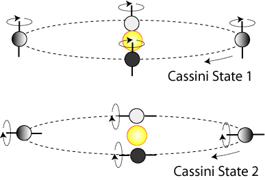
The hot Jupiters that have been observed so far in the infrared using the Spitzer space telescope are all close enough to their parent stars to have been brought into synchronous rotation. That is, their spin periods are the same as their orbital periods and (assuming that they’re in Cassini state #1) they always present the same hemisphere to the star. The weather on these planets will be strongly influenced by the presence of a permanent day side and a permanent night side.

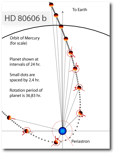
HD 80606b is different. Tidal forces arising during the periastron passages of its 111.4297 day orbit will have brought it into a state of pseudo-synchronization, in which the spin frequency is ~82% of the instantaneous orbital angular frequency that the planet has as it whips through periastron. More precisely, Piet Hut, in this paper from 1981 shows that,

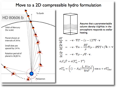
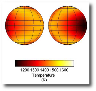
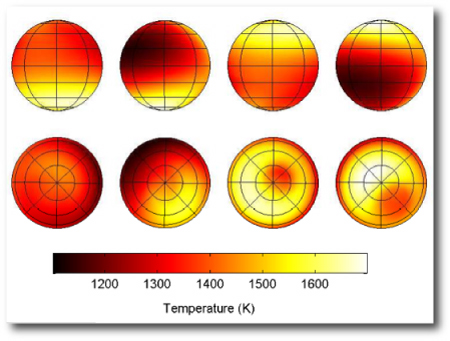
Plugging in 111.4297 days for HD 80606b’s orbital period and e=0.937 for its eccentricity, we get a spin period of 1.535 days, or 36.8 hours. We’re thus in position to understand how the surface of the planet is exposed to intense stellar irradiation during the periastron passage. From this, as we’ll show in upcoming posts, we can make predictions about what Spitzer will see if it observes the star during the time surounding periastron. The geometry looks like this:

In the above diagram, the sense of the orbit is counterclockwise, and the position of the planet is shown at successive 24-hour intervals. If we were to observe from a fixed longitude on the planetary sphere (shown as the red bar at Noon on the leftmost planetary position) then we spin through 235 degrees worth of rotation every 24 hours. At the end of the first 24-hour period, we’re still on the night-side of the planet. During the second 24-hour period, our spot receives it’s strongest heating, and, because of the orbital motion, the day on the equator lasts considerably longer than the usual 18.4 hours. Our spot then receives more than 24 hours worth of darkness to cool off. It’s on the night-side as the planet makes its closest approach to the star. Shortly before dawn during this 24-hour interval, our own Sun crosses the local meridian, an totally inconspicuous 9th magnitude star shining down onto the turbulent steam-choked atmosphere.

Gift idea for ‘606 day

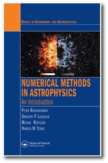
Tis the season! If you’re like me, you’re probably looking for ways to minimize your exposure to malls, crowds, and overloaded sleighs. If so, we here at oklo have devised a one-stop solution for all of your holiday gifts. On Dec. 11th, Taylor and Francis publishers is releasing Numerical Methods in Astrophysics, by Peter Bodenheimer, Michal Rozyczka, Hal Yorke, and myself.

From the publishers description:

This guide develops many numerical techniques for solving major astrophysics problems. After an introduction to the basic equations and derivations, the book focuses on practical applications of the numerical methods. It explores hydrodynamic problems in one dimension, N-body particle dynamics, smoothed particle hydrodynamics, and stellar structure and evolution. The authors also examine advanced techniques in grid-based hydrodynamics, evaluate the methods for calculating the gravitational forces in an astrophysical system, and discuss specific problems in grid-based methods for radiation transfer. The book incorporates user manuals and a CD-ROM of the numerical codes.

It should start shipping Dec. 11th, order yours today!

Watch the Skies

sunset

Image Source.

Sorry about this long lapse in new posts. The end of the academic quarter has left me awash in deadlines and scrambling to get everything done.

Nevertheless, we’ve been making progress behind the scenes. The new oklo server has been delivered, configured, and slotted into a rackspace in a dedicated server room. To use the vernacular, it’s hecka fast. Over the next several days, we’ll be transferring the site over to the new machine, and then it’ll be bye-bye bluehost.

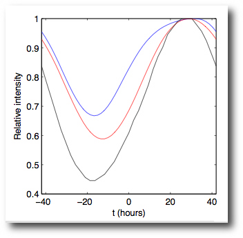
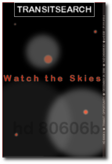
HD 80606 is looking more interesting all the time. I’m working on a writeup of what we’ve been learning. It really has the potential to give us an unambiguous value for the radiative time constant appropriate to the atmospheres of hot Jupiters. The next ‘606 day is December 26th, and I’ll be sending out a circular to the transitsearch.org observers to get a definitive confirmation that it doesn’t transit. Here’s the promotional poster (inspired by the SAO Moonwatch program, while simultaneously attempting to achieve a retro cold-war-flying-saucers feel):

Finally, keep fitting the last batch of Systemic Jr. systems. We need to get a full range of good fits for all of the data sets in order to carry out some very interesting analyses…

New worlds to conquer

Image Source.

The California Carnegie planet search team posted a data-rich paper on astro-ph this week. The new article is scheduled to appear in the February 2007 issue of the Astrophysical Journal. Eugenio, exercising his usual diligence, has added the new velocity tables to both the downloadable systemic console and the systemic back-end stellar catalog.

The highlight of the paper is a new two-planet system orbiting HIP 14810, a metal-rich solar-mass star lying 53 parsecs away. The inner planet in the system has a period of 6.66 days, and tips the scales with least 3.84 Jupiter Masses. The outer planet is less massive (Msin(i)=0.76 Mjup), and goes around the star every 95.3 days.

The secular interaction between the two planets compels them to trade angular momentum back and forth. As a result, the inner planet cycles between an eccentricity of 0.02 and 0.15 on a relatively short 5000-year timescale. It’s currently in the high-eccentricity phase of its orbit. The large radial velocity signal-to-noise for the planet means that its eccentricity can be measured quite precisely (have a look at it with the console). The fact that the orbit is clearly non-circular would be strong evidence for the presence of planet c, even if there weren’t enough data to detect c directly. If planet b was the only significant planet in the system, its orbit would have circularized via tidal dissipation on a timescale that is less than the age of the star.

Short-period planets with masses greater than three Jupiter masses are intrinsically rare. Tau Boo b (with a mass of at least 3.9 Jupiter masses and an orbital period of 3.3 days) is the only other object with roughly similar properties. By contrast, 32 planets with periods of less than a week and minimum masses less than Jupiter’s mass are currently known.

In my opinion, the two most robust statistical correlations that have emerged from the first decade of extrasolar planet detection are (1) the planet-metallicity connection and the (2) dearth of high-mass short-period planets. The planet-metallicity correlation makes perfect sense. It’s the natural, expected outcome of the core-accretion process and the fact that Jovian-mass (as opposed to Neptunian-mass) planet formation is a threshold phenomenon. The paucity of high-mass short-period planets, on the other hand, is both weird and completely unexplained. It’s telling us something about the process of planetary formation and migration. We just don’t know what it is.

Noise Floor

concrete sky

Image Source.

Giant planets are interesting. Terrestrial planets are more interesting. Habitable terrestrial planets are the most interesting of all, and it’s nearly guaranteed that we’re living in the age when the first genuinely Earthlike worlds beyond our solar system will be discovered. The only question is which technique will wind up doing it. The big money is on space-based transit photometry, but I think that ground-based RV might take the prize.

The Systemic Challenge 004 system was designed to be a futuristic idealization of what the Sun’s reflex velocity would like if it were observed with high precision from a neighboring star for more than two decades.

The individual radial velocity uncertainties for the 1172 velocities the Challenge 004 datset are each of order 10 centimeters per second. Errors this small are still safely smaller than the sub-meter per second precision that is currently being obtained by the Swiss team (with HARPS) and the California Carnegie team (at Keck). Given the rapid improvement in the radial velocity technique over the past decade, however, it’s not at all unreasonable to expect instrumental precisions of 10 cm/s fairly soon. Many console users were able to extract the four largest-amplitude solar-system planets — Jupiter, Saturn, Earth, and Venus — out of the challenge004 dataset, suggesting that it’s only a matter of time before instrumental precisions and observational baselines arrive at the threshold where truly habitable, Earth-mass planets can be detected from the ground using the radial velocity technique.

A potential show-stopper for this rosy predictive picture is the astrophysical radial velocity noise produced by the stars themselves. If you want to detect a planet with the mass and period of Earth (which induces a radial velocity half-amplitude of only 9 cm/sec) then you need to be assured that the star is quiet enough for the low-amplitude terrestrial planet signal to be detectable. It’s therefore natural to ask the question: what does the Sun’s reflex velocity look like?

The GOLF experiment on the SOHO satellite provides one set of measurements. A massive time-series of radial velocity observations (from 1996 through 2004) has been published, and is now publicly available. The data set contains over seven million radial velocities taken at a 20-second cadence. The main goal in obtaining this data was to study the Sun’s spectrum of p and g-type modes, which show strongest oscillations at periods of a few minutes.

Three alternate calibrations of the GOLF dataset are posted on the project website. Two of these have clearly been processed to filter out low-frequency, long-period radial velocity variations. It’s interesting, however, to look at what the one unfiltered dataset suggests is happening over timescales of a year or more. I sampled the unfiltered data at a cadence of one velocity measurement per several days, and then loaded the resulting time-series into freshly downloaded version of the systemic console:

radial velocities from the GOLF experiment

According to the above time series, the Sun is a pretty noisy star. I scoured the papers on the GOLF site, and could not find any discussion regarding how much of the variation shown above is believed to come from instrumental effects and how much is belieived to be actually intrinsic to the Sun. The fact that both the scatter and the amplitude of the variations seem to be increasing during the run of the data tend to indicate that intrumental effects relating to the aging of the detector play an important role. If anyone has more specific information on this issue (or if anyone is aware of a preferred calibration) please post to the comments section of the post.

What happens to the detectability of planets that are placed in the GOLF time series? To date, the most precise RV detection of an extrasolar planetary system is the Swiss Team’s discovery of the three Neptune-mass planets orbiting HD 69830. As a control experiment, we relabeled the published HD 69830 dataset at systemic003, and placed it on the backend for Systemic users to evaluate. As expected, nearly all of the twelve submitted fits recovered the published configuration, with chi-square reaching down to about 1.20.

For the systemic004 system, we took the published HD 69830 3-planet orbital model and integrated it forward in time to make a synthetic radial velocity curve. We then perturbed this curve with noise values drawn from the unfiltered GOLF dataset (We averaged the velocities into 15-minute blocks to simulate rapid-fire multiple observations that average over high-frequency p-modes). As of Sunday night, there have been 21 fits uploaded for systemic004 [thanks, y’all, -ed.]. None of them manage a chi-square below 2.5, and aside from the innermost planet, none of them make a convincing case for the presence of the planets that were placed in the dataset. Log in to the backend, call up systemic004 from the “real stars” catalog, and you’ll see what I mean.

The conclusion, then, is that if the GOLF data-set gives a realistic determination of the intrinsic radial velocity variation of the Sun, then the Sun is a far noisier star than HD 69830 (and other similarly old, early K-dwarfs). Indeed, you would even be hard-pressed to believe the presence of Jupiter in the GOLF time-series, unless you’ve got the luxury of waiting for at least several Jovian orbital periods.

dialing 411

Image Source.

Update: The original version of this post tagged systemic003 as the target system and systemic004 as the control system. It’s actually the reverse. In any case, we’re interested in getting multiple fits to both systems. -GL

No post today, just a request:

We’ve been doing an analysis of the detectability of low-mass planets around certain types of stars. In the course of this work, we’ve generated a radial velocity data set, systemic004, which may (or may not) harbor a planetary system. I’d like to ask everyone to (1) download the latest version of the console, and (2) submit your fits to the systemic004 system to the backend. We’ve also included a control system, systemic003, which may look familiar. It would be very useful to have your fits to that system as well.

Thanks in advance! Once we get a batch of fits, I’ll write a post that explains the motivation underlying this request…

year 2.0

Image Source.

As of tomorrow, oklo.org will have been on the air for one year. We’re pleased with the response that we’ve gotten thus far, and we’re looking forward to rapid progress during year two. A big thank-you is definitely in order to everyone who’s either worked on the site or made regular visits or participated in the ongoing collaborative research!

In recent weeks, the user base on the systemic back-end has grown substantially, and we’ve been pushing the limits of what our ISP is geared to provide. Bluehost provides a very cost-effective package for hosting weblogs and running small-scale sites, but it’s become abundantly clear that one can’t expect to run a web 2.0 startup for $6.95 per month. At that level of expenditure, we’ve been limited to the use of 20% of one processor with a maximum job length of 60 seconds. Stefano has stretched our ration with clever use of cron command, but nevertheless,

has become a refrain tiresomely familiar to backend users, and our attempts over the past week to shift the backend to alternate stop-gap servers have been thwarted by various software incompatabilities.

I’m thus very happy to report that an order has been placed for a dedicated server that will obliterate the current problems. It will be located in downtown Santa Cruz on a high-speed T3 line. We should have everything up and running on it within 2 weeks. It’s spec’d to run the full systemic simulation, the new connection is ready to handle a hoped-for shout-out from boing-boing or slashdot, and the joint package should deliver a much more satisfying end-user experience.

In the meantime, however, keep sending in those fits. Neither sleet, nor snow, nor server overloads shall… We’re very eager to build up a solid distribution of fits for Systemic Junior.

Viewed from afar (Challenge 004)

Image Source.

The fourth systemic challenge turned out to be somewhat less challenging than the first three. Quite a few entrants figured out that the data-set corresponds to our own solar system. Among a large number of excellent models, Mark Kilner turned in the fit with the lowest chi-square: 1.0401. In addition to Jupiter, Saturn, Earth, and Venus, he topped off his system with a spurious Mercury-mass planet in a 5.62 day orbit, which allowed him to take the prize. Nice one, Mark!

Eugenio created the challenge 004 synthetic data set after a conversation in which we decided that it’ll soon be feasible to push the precision of the radial velocity method down to an instrumental error of 0.1 m/s. Even more optimistically, we assumed that the Sun, viewed from afar, exhibits negligible radial velocity noise (more on that soon).

Our Solar System, expressed in the Jacobi orbital elements used by the console, is given by:

The true three-dimensional model that Eugenio actually integrated to produce the synthetic data set also includes the correct values for the planetary inclinations and nodes. Because of the sin(i) degeneracy for Keplerian orbits, the current version of the downloadable systemic console does not include the inclinations and nodes as fitting parameters.

The synthetic data set was created with the KeckTAC program, which mimics realistic observing strategies. In an all-out effort on a particular star, one would combine repeated individual observations to get a composite observation that averages over the effect of short-period oscillations (p-modes) of the star itself. This is the strategy that is being currently used by the Swiss team in their campaigns on stars such as HD 69830 and HD 160691. In the challenge004 dataset, there are 1171 radial velocity measurements spread out over 24 years.

Eugenio describes the procedure he used to fit the data:

The periodogram (and the data) shows Jupiter clearly. Saturn appears as a trend, but the periodogram of the residuals after fitting Jupiter gives a good guess for Saturn’s period. After removing Saturn, Earth pops out in the residuals periodogram. I did not find it easy to fit Jupiter, Saturn, and Earth, but after succeeding, Venus very clearly appears in the residuals. I kept on fooling around with the 4-planet fit to see if there was any chance of finding Mars even though the RMS was telling me that 4 planets was the best that I would likely do. I was hoping that N would be large enough to let me get Mars, but I was not able to see a (significant) signal in the residuals periodogram. If anything, Mercury seemed to be more easily detectable. However, after fooling around with the eccentricities of Saturn, Earth, and Venus, the (weak) signal for Mercury disappeared.

Image Source.

With the contests wrapped up, we’re now in the business of getting the fits completed for the Systemic Jr. data set. Eugenio recently incorporated an F-test module into the console, which can be used to determine whether the addition of a planet is warranted. We’ll have a post up shortly that explains in detail how this works. In the meantime, see the discussion on the backend, or download a new console and give its new modules a whirl.

Inky Black Dot

Image Source.

It was a brilliantly clear November afternoon today, and the fact that the Sun’s rays were diminished by 0.0026% mattered not one jot. Mercury was in transit.

I was fortunate to get a glimpse of the event through a telescope. It was about an hour before third contact, and Mercury was clearly visible as a tiny, perfectly round, perfectly black dot set against the pale yellow immensity of the solar disk. There was something about the simplicity of the situation that was quite striking.

Transits, with their odd cadences, link the timescales of human activity to the flow of astronomical time. The June 2004 transit of Venus, for example, took place on the day before the final exam for my introductory Astronomy class. In the weeks leading up to the exam, I would point to Venus shining in the early evening sky, and urge the students to study, “See how it’s getting noticeably lower in the Sky every night at sunset? You can use the angular distance between Venus and the Sun as a countdown clock to the final!” (At which point they’d roll their eyes.)

The next Venus transit is in 2012. The one prior to 2004 took place in 1882, when William Harkness wrote,

We are now on the eve of the second transit of a pair, after which there will be no other till the twenty-first century of our era has dawned upon the Earth, and the June flowers are blooming in 2004. When the last transit season occurred the intellectual world was awakening from the slumber of ages, and that wondrous scientific activity which has led to our present advanced knowledge was just beginning. What will be the state of science when the next transit season arrives, God only knows. Not even our children’s children will live to take part in the astronomy of that day. As for ourselves, we have to make do with the present.

Accurate weather predictions are good for no more than a few days, but transit predictions can be made a long time in advance. For example (according to the Wikipedia) simultaneuous transits of Mercury and Venus will occur in the years 69163 and 224508.

Motions in the inner solar system are nevertheless chaotic, though, with a Lyapunov timescale of order several million years. Our lack of absolutely precise knowledge regarding the positions of the planets at the present moment gradually exponentiates into much larger uncertainties. As a result, we can predict transits millions of years into the future, but we have no ability to predict when the transits of hundreds of millions of years from now will occur.

In fact, there’s even a (thankfully small) chance that the solar system will become dynamically unstable before the Sun swells into a red giant. This afternoon, Mercury seemed utterly insignificant and completely remote when pitched against the solar disk. In the final hours before a collision with the Earth, however, it would present an altogether different sort of impression.