Exoplanet Data Explorer

Competition keeps everyone on their toes, and the exoplanet Doppler detection game is no exception.

The California Planet Search has recently done a major overhaul of their exoplanets.org website, and the results are impressive. The redesigned site is now fully interactive, and it must be seeing a lot of traffic. Certainly, I can count myself as a frequent visitor!

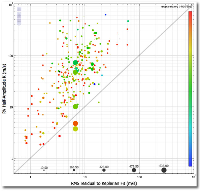
Perhaps the most exciting feature of the site is a plotting applet that seamlessly connects to an up-to-date and curated database of the known extrasolar planets. In the “advanced” mode, one can get very finely tuned plots that can tell interesting stories. As an example, here is a plot of RV half-amplitudes of the known planets plotted against the RMS of the residuals to the fits. The color of the points corresponds to discovery year (cool = back in the day) and the size of each point corresponds to the number of published RV data points for the planet (those five big points correspond to 55 Cancri b-f which has a very extensive data set).

The plot shows that progress comes in part from competition. As the competing Doppler surveys push to lower Ks, there has a been a trend toward decreased signal-to-noise for the detections. It looks like oklo.org posts a few years from now will likely be discussing systems with K~60 cm/sec. At that amplitude, one is plausibly talking habitable worlds.

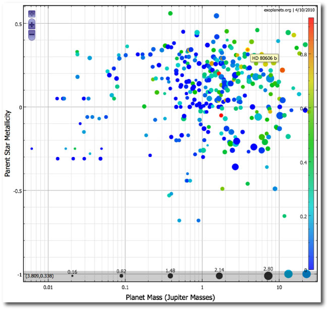
Another interesting plot comes from plotting parent star metallicity against planet mass. As with most of the interesting diagrams, a logarithmic scaling is required. The parent star masses are keyed to the sizes of the individual points, and color is assigned to eccentricity. The software has the nice feature that a cursor placed on a dot informs you of the planet name. This plot shows the benefit of looking at lower mass stars, and it shows how the metallicity correlation is diminished as one pushes below roughly a Saturn mass (evidence, of course, for core accretion):

The exoplanets.org site also contains a very useful planet table, which is giving the competition (in this case, exoplanet.eu) a run for its money.

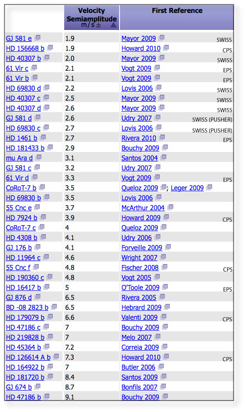
The question of how the world’s top Doppler teams match up in league play is something that I imagine comes up quite a bit in exoplanet-related water-cooler discussions. A suitable scoring system is therefore in order, and the tables on exoplanets.org make this a very doable proposition.

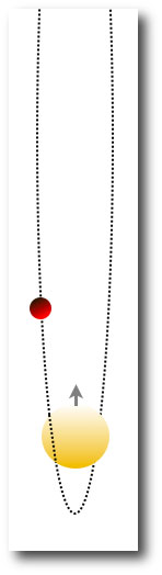
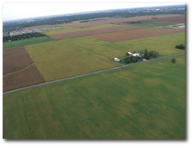
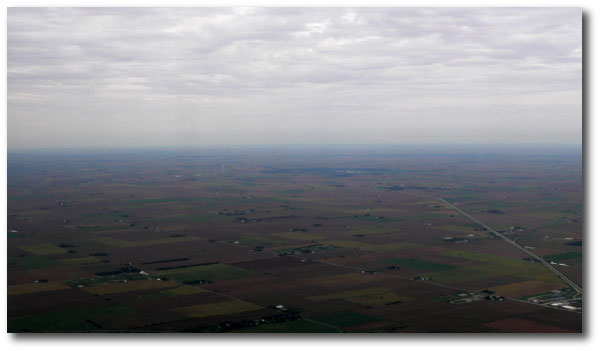
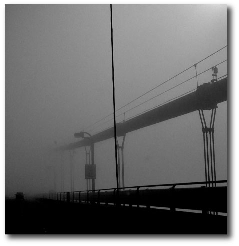
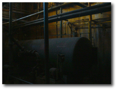
After some thought, I’ve decided to adopt the system used for cross-country running, with the K‘s of the team’s planets replacing the times of the team’s runners. (The image for this post is from a 1983 dual meet between two high school teams from Central Illinois. If you look carefully, you can see that the coach is hurling an acorn at yours truly, presumably because of the much wider-than-expected gap between runners #2 and #3.) In the exoplanet context, the cross-country scoring system encourages fluid changes of lead — one or two high-grade multiple super-Earth systems can catapult a team to the top of the board. From the wikipedia article:

When two or more teams of cross country runners compete, a score may be compiled to determine which team is the better. Points are awarded to the individual runners of eligible teams, equal to the position in which they cross the finish line (first place gets 1 point, second place gets 2 points, etc). Teams are considered ineligible to score if they have fewer than the meet’s required number of scorers, which is typically five. Only the first five runners in for a team are counted towards that team’s score; the points for these runners are summed, and the teams are ranked based on the total, with lowest being best. In the event of a tie, the rules vary depending on the competition; often the team that closes scoring first wins, though in the US NCAA ties are possible. In high school competition, if two teams tie, then the victor is decided by whose sixth runner, the first one whose score does not count, finished first.

The lowest possible score in a five-to-score match is 15 (1+2+3+4+5), achieved by a team’s runners finishing in each of the top five positions. If there is a single opposing team then they would have a score of 40 (6+7+8+9+10), which can be considered a “sweep” for the winning team. In some competitions a team’s sixth and seventh runner are scored in the overall field and are known as “pushers” or “displacers” as their place can count ahead of other runners. In the above match, if there are two non-scoring runners and they came 6th and 7th overall, the opponent’s score would be 50 (8+9+10+11+12). Accordingly, the official score of a forfeited dual meet is 15-50.

According to the above rules, there are currently three RV teams in the running. The Geneva Extrasolar Planet Search (whose planets I’ve listed with SWISS on the table), the California Planet Search (planets listed with CPS), and the Earthbound Planet Search (who I’ve marked as EPS):

The score as of this morning? SWISS 25, EPS 47, CPS 62…

HAT-P-13: good news and bad news


So when presented with that particular formulation, I generally prefer to get the bad news first:

Stefano Meschiari and I have investigated how the new radial velocity data for the HAT-P-13 system affect the possibility of measuring transit timing variations for the short-period planet “b” as the heavy, long-period planet “c” rumbles through its periastron passage later this spring.

First, recall the overall set-up. HAT-P-13 was discovered in transit by Gaspar Bakos and his HAT Net collaborators last summer. HAT-P-13 “b” is a standard-issue hot Jupiter with 0.85 Jupiter masses and a fleeting 2.916-day orbital period. The radial velocity follow-up indicated that the system also contains an Msin(i)~14.5 Jupiter mass object on an eccentric orbit with a P~430 day period. If the two planets are close to coplanar, then the system should have tidally evolved to an eccentricity fixed point — a configuration that allows one to extract Juno-mission style interior information from the inner planet for free.

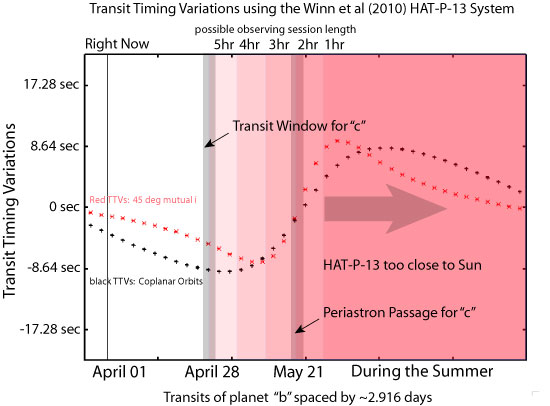
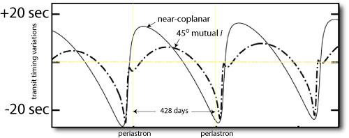
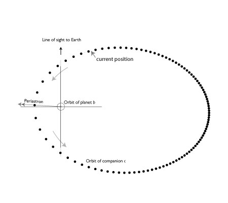
System Version 1.0 for HAT-P-13 generates significant transit timing variations for the inner planet during the weeks surrounding the periastron passage of the outer planet. In a post two weeks ago, I showed some invigorating calculations by Matthew Payne and Eric Ford, which charted the details of the timing variations. Here’s a figure inspired by the Payne-Ford analysis that uses the systemic console’s TTV routines to zoom in on the imminent HAT-P-13 periastron:

The above picture is quite rosy, at least as far as the outlook for TTVs is concerned. With orbital models that are based on the Bakos et al. discovery data for the system, the transit-to-transit time intervals for planet b veer from ~17 seconds shorter than average to ~17 seconds longer than average (relative to the long-term mean) as planet c runs through its periastron and exerts its maximum perturbing influence. This shift from a compressed period to an expanded period occurs rather abruptly over a span of about 2 weeks. Most provocatively, there are significant and feasibly observable differences between the TTV profiles produced by the coplanar configuration and by the configurations with 45-degree mutual inclinations. And finally, all the action was predicted to occur just before the end of HAT-P-13’s yearly observing season (see Bruce Gary’s revived AXA page for wealth of additional detail). It’s not hard to revel in the thought of all the ground-based observers pooling their results (in the spirit of 1761 and 1769) and emerging with a big-picture result!

The new Winn et al. data, however, definitely rain on the TTV parade. The augmented (out-of-transit) data set now shows that the period of planet c is about 20 days longer than previously believed, and c’s eccentricity also drops slightly, from e_c=0.69 to e_c=0.666. With the new orbital model, the differences in the TTVs generated by the co-planar and mutually inclined configurations are considerably smaller. The overall amplitude of the variations is cut nearly in half, and the excitement is pushed far more precariously against the end of the observing season:

And the good news? As described in the last post, the Winn et al. data show that the orbital plane of planet b is probably aligned with the equator of the parent star, which, in turn, means that it’s quite likely that the b-c system is indeed coplanar.

If we assume coplanarity, then the system should be at an eccentricity fixed point in which the apsides of the two planets are aligned. A measurement of the eccentricity of planet b then allows the interior structure and the tidal dissipation of planet b to be measured.

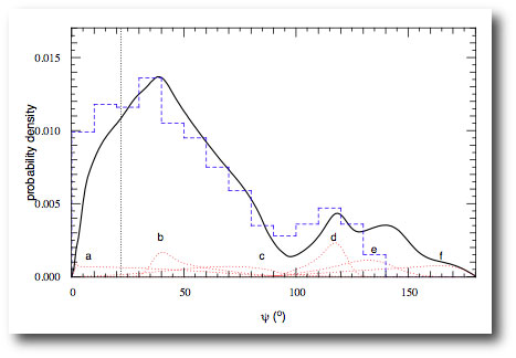
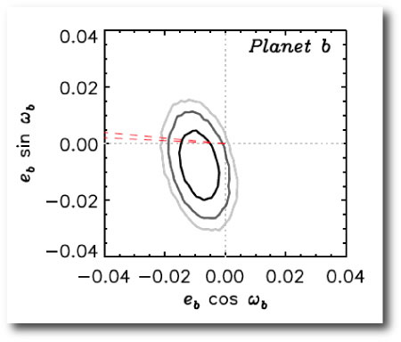
The augmented radial velocity data set permits a better measurement of planet b’s orbital eccentricity. Figure 5 of the Winn et al. paper has the relevant plot, which shows the distribution of Markov-Chain models for the eccentricity and apsidal angle of planet b. If the orbits are aligned, then the true model needs to fall within the red dotted lines, which mark the position of the (much better determined) apsidal line for planet c. From looking at the figure, the apsidally aligned configurations seem to have e_b ~ 0.01±0.005.

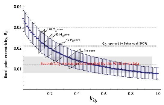
I asked Josh if he could send a histogram that shows the distribution of eccentricities for planet b for the subset of models that satisfy the alignment criterion. He got back to me very quickly with the following plot:

The result is: e_b = 0.0106 ± 0.0040, which implies a best-guess planetary structure that has (1) a small core, (2) a Love number k_2~0.34, and (3) a tidal dissipation quality factor Q~10,000 (see our paper, Batygin, Bodenheimer & Laughlin 2009 for details).

This just in…

With HAT-P-13c rapidly coming ’round the mountain, there was a very timely update on astro-ph last night. Josh Winn and his collaborators have obtained an additional slew of radial velocities which (1) demonstrate using the Rossiter-McLaughlin effect that the inner planet b’s orbit is likely well aligned with the stellar equator, (2) modify the orbital parameters, including the period of the outer massive planet, and (3) hint at a third body further out in the system.

How do these updates affect the unfolding story?

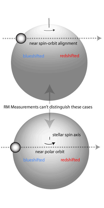
The Rossiter-McLaughlin measurement gives an estimate of the angle λ = -0.9°±8.5°, which is the angular difference between the sky-projected orbital angular momentum vector and sky-projected stellar spin vector. A non-intuitive mouthful. If we’re viewing the star edge-on, then λ = -0.9° amounts to a determination that the planet’s orbital plane is well-aligned with the star’s equator. (See this post for a discussion of what can happen if the star’s rotation axis is tipped toward the Earth). The good news from the measurement is that it’s a-priori more likely that planets b and c are coplanar — that happy state of affairs which will permit direct measurements of planet b’s interior structure and tidal quality factor. If, on the other hand, the planets b and c have a large mutual inclination, then b’s node will precess, and measurement of a small value for λ will occur only at special, relatively infrequent, times during the secular cycle. A close to co-planar configuration also increases the likelihood that the outer planet can be observed in transit.

With their beefed-up data set of out-of-transit Doppler velocities, Winn and his collaborators are able to get a better characterization of the planetary orbits. The best-fit orbital period and eccentricity of the outer planet are slightly modified when the new data are included. The best-guess center of the transit window for c has “slipped” to April 28, 2010, with a current 1-σ uncertainty of 2 days.

The later date, however, is not an excuse for procrastination! Measuring the TTV for this system is a giant opportunity for the whole ground-based photometric community, and a definitive result will require lots of good measurements of lots of transits starting now (or better yet, last month.) I’ll weigh in in detail on this point, along with the challenge posed by Mr. D very shortly…

Inside Information

HAT-P-13c could easily wind up being 2010’s version of HD 80606b — a long-shot transit candidate that pans out to enable extraordinary follow-up characterization, while simultaneously allowing small-telescope ground-based observers to stunt on the transit-hunting space missions.

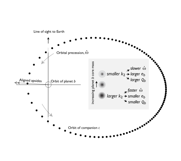
The HAT-P-13 system has already gotten quite a bit of oklo.org press (see articles [1], [2], and [3]). It generates intense interest because it’s the only known configuration where a transiting short-period planet is accompanied by a long-period companion planet on an orbit that’s reasonably well characterized by radial velocity measurements. Right after the system was discovered, we showed that if the orbits of the two planets are coplanar, then one can probe the interior structure of the transiting inner planet by getting a precise measurement of its orbital eccentricity. The idea is that the system has tidally evolved to an eccentricity fixed point, in which the apsidal lines of the two planets precess at the same rate. Both the precession rate and the inner planet’s eccentricity are single-valued functions of the degree of mass concentration within the transiting planet.

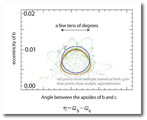
Early this year, Rosemary Mardling expanded the analysis to the situation where the two planets are not orbiting in the same plane (her paper here). If there is significant non-coplanarity, the system will have settled into a limit cycle, in which the eccentricity of the inner planet and the alignment angle of the apsidal lines cycle through a smoothly varying sequence of values. The existence of a limit cycle screws up the possibility of making a precise statement about planet’s b’s interior, even if one has an accurate measurement of the eccentricity.

When one ties all the lines of argument together, it turns out that there are two different system configurations that satisfy all the current constraints. In one, the planetary trajectories are nearly co-planar, with the inclination angle between the two orbits being less than 10 degrees. If the system has this set-up, then we’ll be in good position to x-ray the inner planet. In the alternative configuration, the orbital planes have a relative inclination of ~45 degrees, and the limit cycle will hold.

Matthew Payne, a postdoc at Florida, along with Eric Ford, have done a detailed examination of the transit timing variations that the two configurations will produce. (Transit timing variations — or TTV as all the hipsters were referring to them last week at SXSW — have been all the rage during the last few years, but have so far generated more buzz than results. That should change when HAT-P-13 takes the stage.) Payne and Ford found that timing variations should amount to tens of seconds near the periastron of planet c, which should in turn allow a resolution of whether the system is co-planar or not:

HAT-P-13 is a tough system for small-telescope observers to reach milli-magnitude precision at a cadence high enough to accurately measure the transit timing variations. Nevertheless, the top backyard aces will be giving it a go. Bruce Gary has reactivated the AXA especially for the event, and University of Florida grad student Ben Nelson has written a campaign page for Lubos Brat’s Tresca database. The best transits for detecting TTV will be occurring during April and May. This is an opportunity to really push the envelope.

If the system turns out to be close to coplanar, then there’s a non-negligible probability (of order 5-10%) that planet c will be observable in transit. The transit window is centered on April 12th, and is uncertain by a few days to either side. Small telescope observers will definitely be competitive in checking for the transit. In an upcoming post, we’ll take a look at the details and the peculiarities of this remarkable opportunity.

Cycle 18


It’s been rather arduous past few days as the HST Cycle-18 proposal deadline — 5 PM PST, Friday Feb. 26th, to be exact — bore down like a freight train.

During the past year, I’ve become quite intrigued by the remarkable (and well known) HST observation by Vidal Madjar et al. (2003), who discovered that the Lyman-alpha transit depth of HD 209458b is a whopping 15% (as opposed to the mere 1.5% of the star’s light that gets blocked during the optical transit). The implication of this result is that the planet is surrounded by an outflowing, escaping wind of hydrogen, and the discovery has sparked a lot of theoretical work.

A good test for planetary outflow hypotheses is to see what they predict for eccentric planets that undergo drastic changes in stellar heating during the course of the orbit. Fred Adams and I have been working on hydrodynamical models for these situations, and it soon became clear that oklo.org fave HD 17156b, the P=21.2d, e=0.67 transiting planet provides an intriguing observational opportunity for HST/STIS. HD 17156 is currently the fourth-brightest known parent star of a transiting extrasolar planet (after HD 209458, HD 189733 and HD 149026) and it lies in HST’s so-called continuous viewing zone for part of the year. This means that a full transit can be observed without having to take those leisurely once-per-96-minute pit stops every time Earth blocks the view.

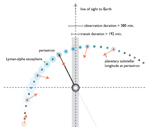
The geometry of the transit, furthermore, is such that the planet is getting its maximum sunburn just a few hours after transit egress. Our calculations indicate that it should take the upper atmosphere only a matter of hours to react to the increased heating, so we’re optimistic about the possibility that not only will HST detect a deep transit in the UV, but that it might even be able to detect the Lyman-alpha transit depth increasing during the course of the transit. Here’s the basic idea:

As of a few minutes ago, the proposal was received safe and sound at STScI, so now it’s time to kick back, wait, and see if it passes muster with the TAC…

upcoming event

I’ve got an upcoming event planned in New York City that should be pretty interesting. From the UCSC Newsletter:

UCSC astronomer joins composer Philip Glass to explore music of the universe

UC Santa Cruz Astronomer Gregory Laughlin joins acclaimed composer Philip Glass February 21 in a “Brainwave” discussion at the Rubin Art Museum in New York.

For its third year and in conjunction with the exhibition Visions of the Cosmos, Brainwave is a series of 20 sessions this winter and spring that bring together eminent thinkers from multiple disciplines with neuroscientists and astrophysicists to ponder big thoughts about “things that matter.”

Laughlin and Glass appear in the third Brainwave event titled “How Do We Listen to the Music of the Spheres?”

Laughlin is a professor of astronomy and astrophysics whose research delves into orbital dynamics and the evolution of planetary systems. Glass is one of the most influential composers of the past half-century. Though sometimes called a “minimalist,” Glass describes his compositions as “music with repetitive structures.”

Laughlin said he and Glass will explore commonalities between music and orbital dynamics. The museum’s initiative to pair the two was sparked in part by Laughlin’s articles on his blog oklo.org that delve into ways to “sonify” planetary movements.

He developed software to map planetary systems as audible waveforms. He said he became intrigued by the realization that planetary systems can be used as a type of nonlinear digital synthesizer and can provide an enormous palette of sound — sounds never before heard.

The Laughlin/Glass Brainwave session begins at 6 p.m. Sunday, February 21 at the Rubin Museum of Art at 150 West 17 St., New York City. Admission is $25.

Over the next week, as I’m preparing for the event, I’ll be working extensively with the sonification capability of the systemic console. Just below, is a reprinted post that touches on this very cool, and still relatively unexplored feature. If you’ve worked with the Console’s N-body sonification, and if you’ve found interesting results, feel free to send me .fit files — an extraordinarily effective form of compression(!) — and I may be able to use them in the discussion.

Potentially the most interesting feature on the downloadable systemic console is the “sonify button”, which integrates the model planetary system specified by the state of the console sliders and produces a .wav format CD-quality audio file of the resulting radial velocity waveform. Not interested in planets? The console is a stand-alone non-linear digital synthesizer. It’s capable of producing strange, remarkable, musically useful sounds. They merely need to be located within the uncountable infinity of solutions to the gravitational N-body problem.

First, use the console to build an interesting multi-planet system (for this purpose, there’s no need to try to fit whatever data is in the window.) Then click the sonify button. This brings up a dialogue window which enables the user to make several specifications for the sound file that is produced.

console sonify dialogue box

The most important user-specified parameter is the frequency onto which the orbital period of the shortest-period planet on the console is mapped. If, for example, the innermost planet has a period of 365.25 days, then a 440 Hz map will play 440 years worth of evolution in one second. (440 Hz corresponds to the A below middle C.) Mapping the radial velocity curve onto a high-frequency note extends the total number of orbits that go into the sample, and thus increases the integration time required to produce the sample. You can also specify the length of the sample, and you can exert simple control over the attack and decay rate of the envelope for the overall waveform.

Once you’ve produced the sound file, it appears in the “soundClips” subdirectory within the systemic parent directory. Both of these directories are automatically created when you download and expand the console — see the instruction set for the downloadable console for more details. With a Macintosh, you get the best results if you play the sample right from the folder. i-Tunes seems to want to convert the samples to .mp3 format in a manner that introduces audible noise, and we’re not yet sure how to resolve this issue.

To the extent that planets orbit independently of one another, the console behaves like a simple additive synthesizer, in which the individual Kepler waveforms add to form a composite sound. Much more interesting, is the situation when planets experience significant gravitational interaction, leading, for example, to resonance and to nonlinear instability (here are examples, 1, 2, from the resources page of both types of waveforms). Close encounters provide discontinuities between individual blocks of sound that resemble the results of granular synthesis.

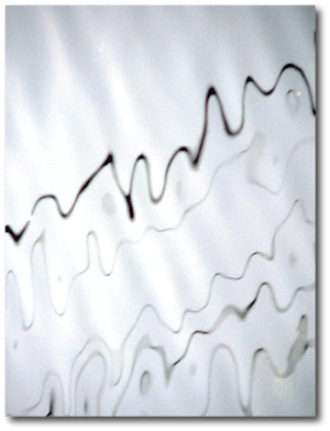
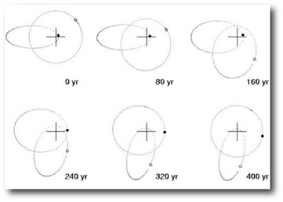
The strongest 2-planet mean-motion resonances occur when the pair of planets share a common period and engage in a one-to-one resonant motion. There are a variety of different one-to-one resonances, including binary planet orbits (e.g. Earth and Moon), trojan configurations, and generalizations of retrograde satellite orbits. In this last category, one can have two planets with the same semi-major axis, but with different eccentricities. If one starts the planets in the following configuration, then the motion is dynamically stable, and evolves in a complicated way over time.

evolution of eccentric 1:1 resonance

The motion leads to an interesting audio wave-form, in which you can hear the system cycling between configurations in which both planets are modestly eccentric and configurations in which one orbit is nearly circular while the other one is highly eccentric. As a specific example, set the console to the following configuration: P1=P2=10 days, M1=M2=0.3 Mjup, MA1=180., MA2=190., e1=0.9, e2=0.1, long1=0.0, long2=0.0. If you increase MA2 to about 225 degrees while keeping the other parameters fixed, you’ll hear the system go unstable.

Evolving, high-eccentricity orbits tend to have an insect-like quality, which brings to mind the 1986 album, The Insect Musicians, by Greame Revell (formerly of SPK). From the album jacket:

For the two years 1984-85, Graeme Revell traveled from Australia to Europe, to Africa, Indonesia and North America recording and negotiating copyrights of insect sound recordings. It took another full year sampling and metamorphosing some forty sounds thus gathered using the Fairlight Computer Musical Instrument, to produce this record. The only sounds used are those of insects, altered digitally and combined into a unique orchestra of instruments, an orchestra of strange and delicate timbres, music of natural rhythm and texture.

limit cycle

The minimum threshold level for amazement will rise quickly once Kepler’s discoveries start to accumulate, and already, it’s getting very hard to remember which transiting planet is unusual for which reason. Let’s see, was it TrES-4 or WASP-17 that had that styrofoam-like density? Or was it both of them?

Even in a crowded field, though, HAT-P-13 is likely to endure as a touchstone. In the next five years, it’s likely that there will emerge only a select handful of systems in which a well-characterized transiting planet orbiting a relatively bright star is being substantially perturbed by a companion on a well-characterized orbit:

After the HAT-13 system was announced, we showed that the planets “b” and “c” should have evolved to an eccentricity fixed point configuration, in which the orbits’ apsidal lines co-rotate, and in which the orbital eccentricity of planet “b” has a very sensitive dependence on its internal structure. Further modeling, using reasonable assumptions, gives strong limits on the tidal Q of planet “b”. In essence, one can potentially accomplish with an exoplanet a big chunk of what the Juno Mission expects to accomplish at Jupiter at of order a thousandth of the cost.

Our analysis assumed that HAT-P-13 b and c are on co-planar orbits. There’s an interesting new paper by Rosemary Mardling that explores the significantly more complex situation that arises if the orbital planes of the planets are significantly misaligned. In this case, tidal dissipation in the inner planet causes the system to settle into a limit cycle, where the eccentricity and the angle between the apsides circulate on a secular timescale, and the easy insight into the structure of planet b is no longer possible.

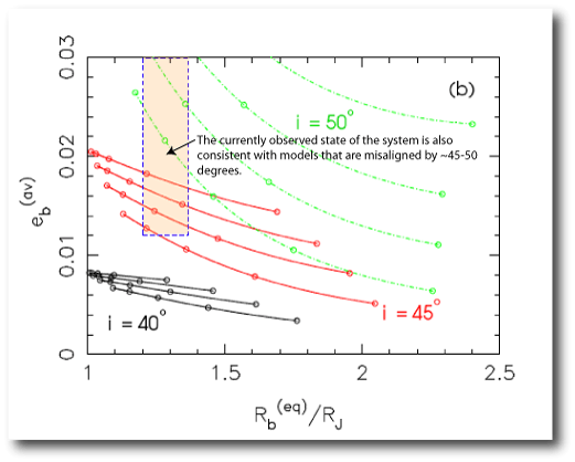
Interestingly, however, Mardling’s analysis suggests that if the orbits are misaligned, then the mutual inclination is likely to be in the neighborhood of 45 or 50 degrees. A mutual inclination of, say, 30 degrees is inconsistent with the currently observed parameters of planet b. The following two diagrams (figure 8 a and b) from her paper show how this works:

Within the next few months, we should get improved values for the eccentricity and radius of planet b, which will significantly shrink the size of the peach-colored boxes in the two figures above. HAT-P-13c is also currently headed in for periastron, with the next transit opportunity scheduled for April 12, 2010. A transit by planet c would provide strong evidence that the system is reasonably close to co-planar (and would be quite remarkable in its own right!) Furthermore, during the periastron passage of c, there should be readily detectable transit timing variations for b, which should give us a shot at distinguishing between the co-planar case and the case with a mutual eccentricity of 45-50 degrees. In the next post, I’ll look in detail at the numbers…

Red Dwarf Metallicities

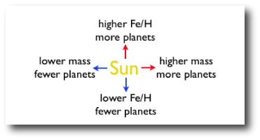
A core prediction of the core accretion model for giant planet formation is that the frequency of readily detectable giant planets should increase with both increasing stellar metallicity and with increasing stellar mass:

It’s now well established that the above diagram is zeroth-order correct, but until fairly recently, the conventional wisdom held that there is little evidence for a strong planet-metallicity correlation among the handful M-dwarf stars (for example, Gliese 876) that are known to harbor giant planets. One is then naturally led to speculate that the odd giant planets in a systems like Gliese 876 might be the outcome of gravitational instability rather than core accretion.

The profusion of molecular lines in the atmospheres of M dwarfs make it hard to determine their metallicities using the techniques of spectral synthesis that work well for hotter stars like the Sun. Fortunately, though, the red dwarfs’ legendary stinginess provides another opportunity for assessing metallicity. Red dwarfs are so thrifty, and they evolve so slowly, that every single one that’s ever formed has barely touched its store of hydrogen. With all the fuel gauges pegged to full, a critical parameter’s worth of confusion is removed. Red dwarfs of a particular mass should form a well-defined one-parameter sequence in the Hertzsprung Russell diagram, and that parameter should be metallicity. If one can accurately plot a particular low-mass star on a color-magnitude diagram, then there should exist a unique and high-quality mapping to both the star’s mass and its metallicity. Physically, an increase in metallicity leads to a higher photospheric opacity, which provides an effective layer of insulation for a star. Add metals to a red dwarf and it will move down and to the right in the Hertzsprung Russell diagram.

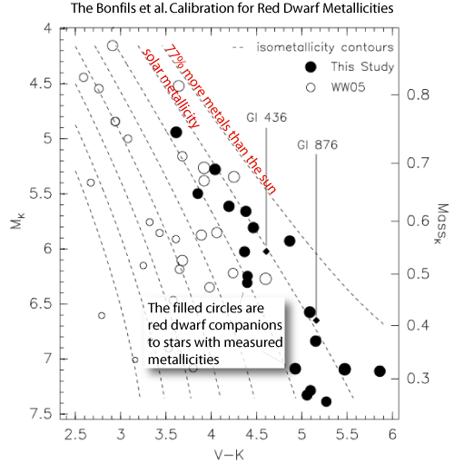
Because of the nightmarish complexity of red dwarf atmospheres, it’s not easy to find the calibration that allows one to make the transformation between an observed absolute magnitude and color index (e.g. M_K and V-K) to the stellar mass and metallicity. In 2005, however, Xavier Bonfils and his collaborators made a breakthrough by employing a simple should’ve-thought-of-that-myself technique: Binary stars generally stem from a common molecular cloud core, and so the members of a binary pair should thus generally have very similar metallicities. In particular, if you measure the metallicity of an F, G, or K binary companion to an M-dwarf, then you can assume that the M-dwarf has the same metallicity. Do this often enough, and you can infer the lines of constant M-dwarf metallicity on a color-magnitude diagram. With the calibration in place, metallicity determinations for field red dwarfs are simply a matter of reading off the nearest iso-metallicity locus. Here’s the key diagram from the Bonfils et al. paper:

The puzzling outcome of the Bonfils et al metallicity calibration was that the rare giant-planet bearing M-dwarfs such as Gliese 876 and Gliese 849 didn’t appear to be particularly metal rich, and that worked to undermine confidence in the core accretion picture. One would naively expect that a low-mass disk will need all the help it can get in order to build giant planet cores before the gas is gone. If anything, the planet-metallicity correlation should be strongest among the M-dwarfs.

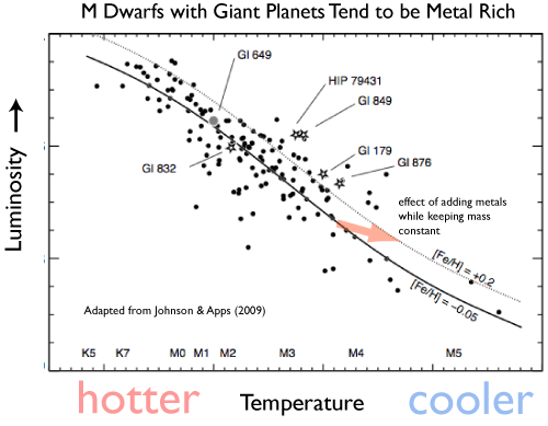
Important recent progress was made last year by John Johnson and Kevin Apps, who published a reevaluation of Bonfil et al’s. isometallicity loci in the color-magnitude diagram. Johnson and Apps point out that application of the Bonfils et al. calibration produces an aggregate of local M-dwarf stars that have a significantly lower average metallicity than that for the local FGK stars. There’s little reason to expect such a dichotomy, which implies that the Bonfils et al. correlation may be systematically underestimating metallicity by roughly a factor of two. No small potatoes!

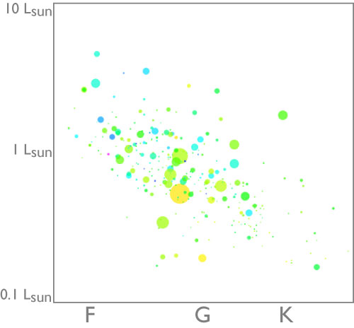
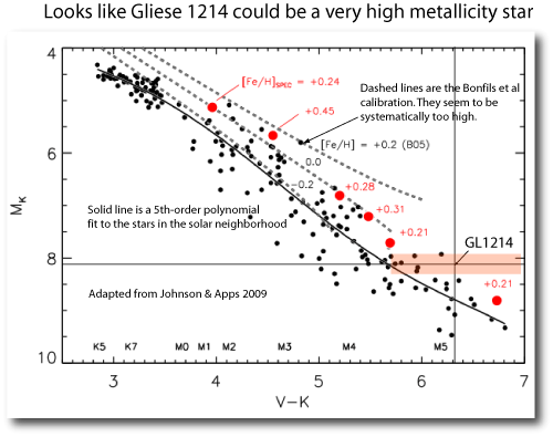
Johnson and Apps adjusted the calibration to bring the metallicities of the local M dwarfs into line with the metallicities of the local FGK dwarfs. Here’s a slightly adapted version of their key diagram:

With the revised calibration, Gliese 876 turns up with a metallicity twice that of the Sun, and there is excellent evidence that the planet-metallicity correlation holds strongly for the M dwarfs that harbor relatively massive planets. Furthermore, it’s hard to argue with the two recent papers (one, two) from the California Planet Survey which report the detection of relatively massive planets orbiting two nearby M dwarfs, both of which have extremely high metallicities with the revised calibration.

The statistics are still small-number, but there’s a strong hint that the planet-metallicity correlation for Neptune and sub-Neptune mass planets orbiting M-dwarfs is stronger than it appears to be at FGK (where it’s effectively non-existent). Gliese 176, and Gliese 436, for example, are both quite metal-rich. I bet that a survey like Mearth could jack up its yield by shading its telescope visits to favor the high-metallicity stars on the observing list…

Indeed, if we plot Gliese 1214 (V=15.1±0.6, K=8.78±0.02, parallax=0.0772±0.0054”, distance modulus=0.562±0.16) in comparison to the stars in the local volume, it looks like Gliese 1214 has of order twice solar metallicity if we adopt the nominal values for V,K and the distance. That’s very intriguing…

Follow Up

Astronomers worldwide staggered into work this morning, some of them rudely elbowing their way to the front of the lines at the espresso machines, clear evidence that events surrounding the January 2010 ‘606 holiday season have finally drawn to a close.

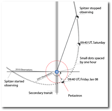
Hopefully the data will turn out to be of high quality! As I mentioned in yesterday’s post, ground observers in both Europe and North America were out in force for the event, collecting photometric and spectroscopic data. The action was covered from space as well. We were awarded a generous 84-hour block of time on Warm Spitzer. The telescope started collecting 4.5-micron photometry more than a day prior to the secondary transit, and ended more than two days after the periastron passage.

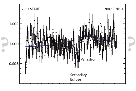
What do we hope to learn? By observing the run-up to the secondary transit, we should be able to establish an improved baseline temperature for the planet, which should afford a better sense of how much tidal heating is occurring. And during the days following periastron, we expect to see a near-complete drop-off in flux from the planet as the periastron nightside hemisphere rotates fully into view. The 2007 observations came to a frustrating end just as this should have been starting to occur.

In addition to the secondary eclipse and the ground-based observations, Guillaume Hebrard and his collaborators were awarded 19 hours on Warm Spitzer to observe the primary transit at 4.5 microns. Their photometric time series will enable an improved radius measurement for the planet — both because of the highly accurate photometry and because the effects of stellar limb darkening are negligible in the infrared. Their time series will establish a very precise ephemeris for the transit, which will enable future observations to monitor the system for orbital precession.

Looking forward to the results…

in eclipse

It’s 4pm Wednesday Jan 13th here in Santa Cruz, and the HD 80606b transit has been underway for a few hours. A whole slew of observers worldwide are watching the event, with Northern Europe getting the best view (if the weather is clear).

Last weekend, the Spitzer telescope carried out an 84-hour observation of the system during the window surrounding the secondary eclipse. Our goal was to watch the planet heat up and then cool down rapidly as the unheated night side rotates into view.

Good luck to everyone who’s out there on the sky!

Kepler’s first crop


The long-awaited initial discoveries from the 600M Kepler mission are in!

At a scientific talk at the AAS Meeting in Washington DC this morning, and in an afternoon press briefing packed with journalists, bright lights and television cameras, the Kepler Team announced the discovery of five new transiting planets. Four are inflated hot Jupiters, and one is a hot Neptune reminiscent of Gliese 436b and HAT-P-11b. Most importantly, the Kepler satellite appears by all accounts to be performing beautifully as it continuously monitors over 150,000 stars for planetary transits.

Here’s a to-scale line-up of the Kepler starting five. Kepler-4b is so small that it’s just barely resolved at a scale where its orbit spans 480 pixels.

The Kepler planets are primarily orbiting high-metallicity, slightly inflated, slightly evolved stars. These particular parent stars were likely selected for high-priority confirmation observations because their abundant, narrow spectral lines should permit maximally efficient, cost-effective Doppler-velocity follow-up.

Among the planets, Kepler-4b, with its composition that’s likely largely water-based, provides further evidence that the majority of short-period planets formed far from their parent stars, beyond the iceline in the protostellar disk, and subsequently migrated inward. Kepler-7b is approximately the density of styrofoam. In a conversation with a reporter, I scrambled for an analogy:

It’s like looking at a football team. You might guess from the team photo that they’re all 250 to 300 pounds. But then you find out that some of them are 25 pounds; that would come as a surprise…

Everyone is looking forward to the big-picture results that will be coming from Kepler a few years hence, as it probes into the habitable zones of Solar-type stars. In the interim, though, the veritable flood of ultra-high precision photometric data arriving via the the Deep Space Network will keep Doppler velocity follow-up observers working the late-night shifts. The parent stars of the new planets are in the V=12.6 to V=13.9 range, roughly 100 times fainter than the prime transit-bearing stars such as HD 209458 and HD 189733.

According to a S&T editor Bob Naeye, who reported on Bill Borucki’s scientific talk this morning, the first 43 days of photometric observations from the satellite generated 175 transit candidates, of which 50 were followed up in detail to extract the 5 announced planets. The Keck I telescope has been the major workhorse for the high-precision RV follow-up efforts that are required to get accurate masses. According to the Keck I Telescope Schedule, 17 nights were allocated to the Kepler team from July through December of last year. Within this time alotment, roughly 50 RV measurements for the 5 new planets were obtained. The velocity precision for Kepler-4b looks to be of order 2-3 m/s, which is excellent. Here are two thumbnails from Borucki’s talk (look carefully to read the y-axis scale):

With a slew of nights and good weather during 2010, it should be possible to get a significant number of additional planets confirmed…

Ringing out the Old Year

Image by JUNe (source)

At the beginning of the year, I made five exoplanet-related predictions:

1. A 1.75 Earth Mass planet orbiting a Main Sequence star.

2. A confirmed case of transit timing variations.

3. A transiting planet in a well-characterized multiple-planet system.

4. A transiting super-Earth (or more precisely, on the basis of observed composition, a transiting sup-Neptune).

5. 417 planets listed on exoplanet.eu.

So how did I do?

Prediction 1 was just a bit on the optimistic side. At present, the extrasolar planet with the lowest Msin(i) orbiting a Main Sequence star is Gliese 581e, with Msin(i)=1.94±0.22 Earth masses. So the forecast panned out to within the 1-sigma error. (Mayor et al.’s discovery paper is here, oklo.org coverage of the discovery is here, here, and here).

Prediction 2 falls just short of unambiguous fulfillment. HAT-P-13b is clearly going to exhibit transit timing variations, and soon, but as discussed in Bakos et al.’s discovery paper, it’s not clear whether they’ve already been observed.

Prediction 3 is satisfied by HAT-P-13b and c. The characterization is so good, in fact, that we’re able to effectively look inside HAT-P-13b.

Prediction 4 was doubly satisfied. First, by CoRoT-7b (a transiting super-Earth), and second, by GJ 1214b (a transiting sub-Neptune).

Prediction 5: 415 planets are listed (as of 12/31/2009) on exoplanet.eu…

BD 08-2823b (or opportunity comes knocking)

I was catching up on astro-ph.EP this morning, and came across Paper #20 from the HARPS Search for Southern Extrasolar Planets. The authors report the detection of two new planets orbiting BD 08-2823, a nearby, moderately active K-dwarf. The inner planet in this new system has a mass comparable to Uranus (Msin(i)=14.4 Earth Masses) and an orbital period of 5.60 days — yet another example from the huge population of super-Earths and sub-Neptunes lying in short-period orbits around the Sun’s closest neighbors. As described in the paper, the two new planets emerged serendipitously from a thwarted attempt to identify transiting planets using the Hipparcos database.

What caught my eye about BD 08-2823b, is the fact that the parent star has not yet been monitored for transits. The a-priori probability that BD 08-2823b can be observed in transit is >7%. The star is observable from both hemispheres, at V=9.86 it’s a natural for small-telescope ground-based observers, and it’s up right now!
A successful detection is no walk in the park: The expected transit depth is of order 1.2 millimag, right at the limit of what’s been demonstrated by skilled small-telescope observers. The possible short-term activity of the parent star will demand multiple confirmations in the event that transits are indeed occurring. The current transit ephemeris is uncertain by more than a day to either side of the predicted transit midpoints (just added to the Transitsearch.org candidates table).

The transit valuation metric (described here) assigns a real-world value to the detection of a given transiting planet. It’s a way of cutting through hype, and it keeps a necessary spotlight on the fact that the cost of detecting a given transiting planet is not necessarily proportional to the scientific value of the planet detected.

If BD 08-2823b transits, its value using the metric works out to ~3 Million dollars. In other words, a detection would amount to a major discovery (something that’s getting increasingly harder to pull off, given this past year’s flood of results). In expectation, factoring in the 7% transit probability, the value is 210K. On a per-night basis, this is well over twice the value of Keck time, and yet it can be had by a good observer with a good backyard telescope. The next opportunities are centered on Jan 1st, and Jan 7th.

Dome

From the short film "Dome" by Tony Misch

Here’s another remarkable YouTube video.

It’s a time-lapse movie that shows the construction of the dome for the Automated Planet Finder Telescope at the Lick Observatory on Mt. Hamilton. The sequence was assembled by Tony Misch (Support Astronomer for Lick Observatory) who created a 3-minute visual narrative by drawing from an archive of 200,000 frames taken at 2-minute intervals between Sept. 15th, 2005, and Aug. 14th, 2006. Be sure to turn up the volume — Paul Alcott’s fine-grained mechanized score is reminiscent of Autechre, and works very well.

The APF telescope will be used by the California Planet Search (CPS) and the Earthbound Planet Search (EPS) projects to carry out high-precision radial velocity monitoring of nearby stars. It’ll start collecting data within the next few months.

A Blue ‘606 Day

The traditional definition of a “Blue” moon is the third Full Moon in a season containing four Full Moons rather than the usual three. In 1946, Sky and Telescope Magazine inadvertently launched a new, somehow more modern definition of a “Blue” moon as the second Full Moon to occur in a calendar month.

On the scale of urgency, the correct definition of a Blue Moon ranks favorably with such matters of astronomical concern as whether Pluto is a planet. I thus have to admit, that I immediately dropped what I was doing to answer a reporter’s e-mail query:

I read several accounts that the phenomenon will occur on New Year’s Eve based on the recent definition. Do you know if that’s accurate?

I answered:

We here in the United States will indeed be having a Blue Moon on New Year’s Eve according to the currently popular definition of a Blue Moon as “the second Full Moon to occur in a calendar month”.

The times at which the Moon is full (which occurs when the Sun, Earth and Moon form a line as viewed from above) can be calculated with great precision and with zero ambiguity. The current set of Full Moon times are:

02 December 2009 at 07:30 GMT
31 December 2009 at 19:13 GMT
30 January     2010 at 06:17 GMT
28 February   2010 at 16:38 GMT
30 March        2010 at 02:25 GMT

GMT stands for “Greenwich Mean Time”. This is the same as Universal Time, and corresponds to the current time zone for England (where the Greenwich Observatory is located). As you can see, for GMT, there are Full Moons in December 2009.

Here in California, we’re currently on Pacific Standard Time, which is 8 hours behind GMT. That means we had a Full Moon on Dec 1st at 11:30 PM, and we’ll have the next one on New Year’s Eve at 11:13 AM in the morning, giving us a Blue Moon.

In Australia, which lies between 8 and 10.5 hours ahead of GMT, the next Full Moon will occur on New Year’s Day, 2010. Australia, therefore, will not be experiencing a Blue Moon on New Year’s Eve, 2009 (the same is true for Japan, China, etc.).

Revelers in the Far East, however, should not feel left out. If you look at the table above, you’ll see that the Far East will experience a “double Blue Moon” in 2010, in which both the months of January and March will contain two Full Moons.

Blue Moons have no astronomical significance. The “Blue Moon” is just a name in the same sense as a “Hunter’s Moon” or a “Harvest Moon”. The Blue Moons are a purely cultural artifact that arise from the juxtaposition of the celestial clockwork of the lunar and terrestrial orbits with the Gregorian Calendar, which was introduced on 24 February 1582 through a papal bull by Pope Gregory XIII, and which has now been adopted worldwide as the standard civil calendar.

Even though Blue Moons have no astronomical significance, there is something oddly appealing about events that stem from the overlap (or better, the “beating”) between the precise orbital rhythms of planets and moons, and the ebb and flow of human-centered events here on Earth. At my weblog, oklo.org, I’ve been promoting a new holiday, ” ‘606 day”, which occurs every 111.43637 days when the wildly eccentric transiting planet HD 80606b makes its dramatic perihelion passage.

The ‘606 days for 2010 will occur on (adopting Universal Time):

Jan 8, 2010 at 9:49 AM
April 29, 2010 at 8:17 PM
August 19, 2010 at 6:45 AM
Dec 8, 2010 at 5:12 PM

In normal years, there are only three ‘606 days. In 2010, however, we’re lucky to have four. This “extra” ‘606 day is analogous to a blue moon.

Happy Holidays!

-Greg

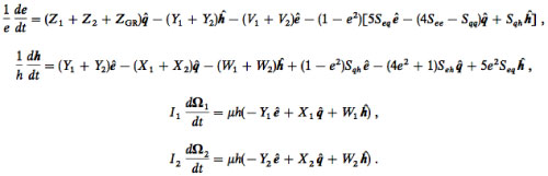
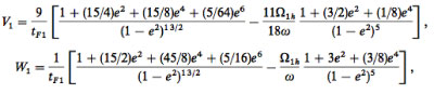
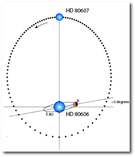
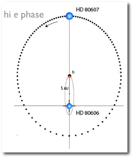
(For readers unfamiliar with HD 80606b and  ‘606 days, see):

http://oklo.org/2009/01/29/the-big-swing/, http://oklo.org/2009/02/08/whats-your-angle/, http://oklo.org/2009/02/12/ready-set/, http://oklo.org/2009/02/12/go/, and http://oklo.org/2009/02/25/hd-80606b-transit-detected/

Update 1/2/10: Here’s a link to a call-in interview that I did on KPCC (L.A. Public Radio). As you’ll hear, there’s one regrettable gaffe where I say that a year contains “thirty days”… Not quite becoming of an Astronomy Professor!