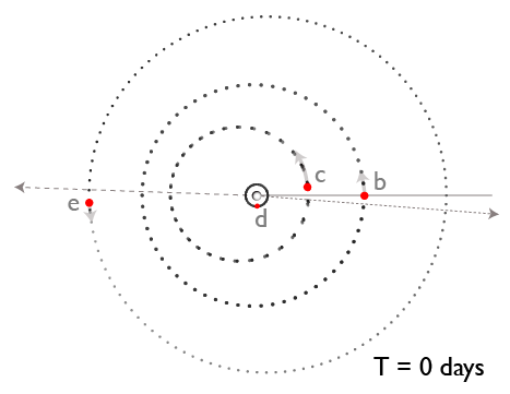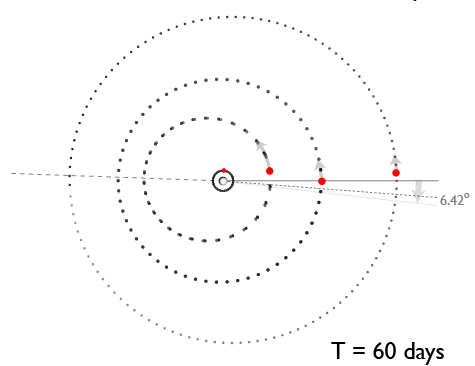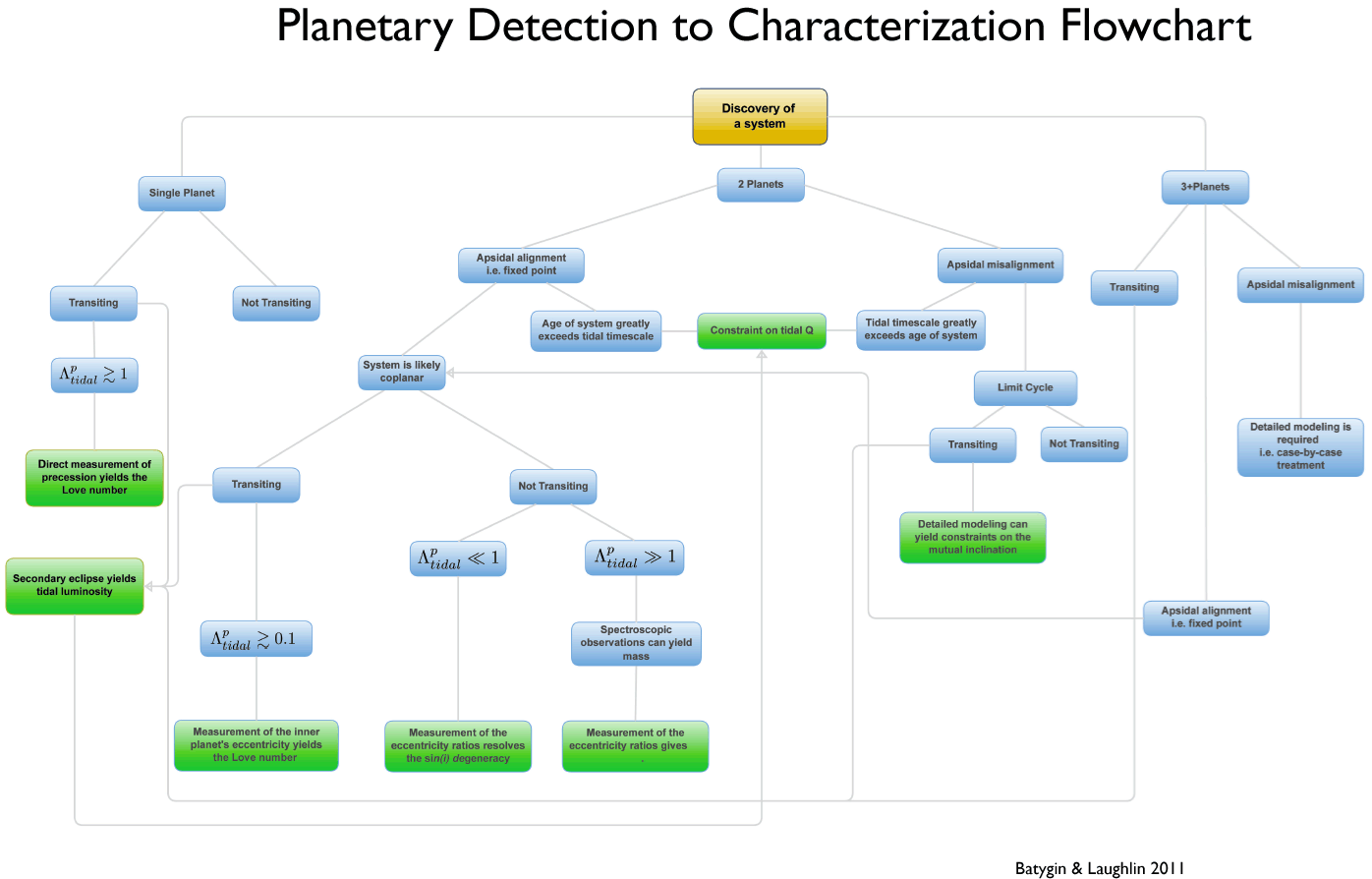
Neptune after one orbit

This coming July, the planet Neptune will have completed one full orbit since its discovery on September 23, 1846, an event which constituted the occasion, a week ago Sunday in Seattle, for a special session of the Historical Astronomy Division of the American Astronomical Society. From the conference program:

The year 2011 marks not only the 200th anniversary of the French mathematical astronomer Urbain Le Verrier’’s birth, but also the first return of Neptune to its optical-discovery position in 1846. Despite the passage of more than 164 years since that planet discovery, the circumstances surrounding the near-simultaneous mathematical predictions of a transuranian disturbing planet made by Le Verrier and John Couch Adams, a young Fellow in St. John’s College at the University of Cambridge, and the subsequent optical discovery of Neptune by German astronomer Johann Gottfried Galle at the Berlin Observatory continue to remain controversial. The double anniversary occurring in 2011 is an appropriate time to examine the Neptune discovery event from a number of new perspectives. In this session we shall explore how Cornwall shaped Adams’ early education and his method of locating the presence of a hypothetical disturbing planet. We shall examine the possibility that Adams (and perhaps Le Verrier as well) may have had Asperger’s Syndrome (high-functioning autism), a condition that may explain their difficulties in communicating and interacting with their contemporaries. The intense French press attack on British astronomers immediately after the discovery is examined in detail for the first time. The role that Benjamin Peirce’s analysis of Neptune’s actual orbit (which differed greatly from those hypothesized by Adams and Le Verrier) played in the development and European perception of American astronomy and mathematics will be discussed. We open and close the session with presentations placing the Neptune discovery event within the context of 19th-century science and relating it to modern-day searches for planets in the outskirts of the solar system and around other stars.


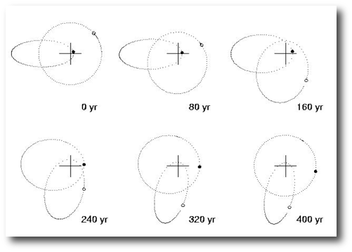
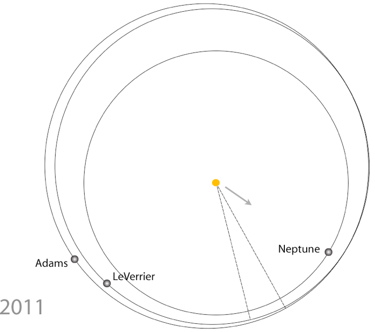
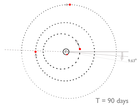
That Benjamin Peirce (pictured above), of the Harvard College Observatory, generally plays no role in the Astronomy 101 narrative of the discovery of Neptune is an interesting object lesson in itself: Nobody likes a playa hater. Peirce pointed out the inconvenient truth that the orbits calculated by Adams and LeVerrier, both of whom relied on Bodes’ law to inform their semi-major axes, are startlingly different from the actual orbit of Neptune:

In Peirce’s view, the discovery of Neptune constituted a “happy accident” because the event took place at the fortuitous time when the longitudes of the predicted and observed incarnations of Neptune lay near the same point on the ecliptic. Fast forward by one orbit, and the predictions don’t fare particularly well in a visual search with a 24.4 cm refractor:

Peirce did have a point. If you use a vague empirical law to inform a prediction, are you justified in reaping the accolades? Indeed, some of the praise that came to LeVerrier might justifiably have been seen as over-the-top:

I cannot attempt to convey… the impression that was made on me by the author’s undoubting confidence, but the firmness with which he proclaimed to the observing astronomers, `Look into the place which I have indicated and you will see the planet well.’

–George Bidell Airy, British Astronomer Royal

This scientist, this genius… had discovered a star with the tip of his pen, without other instrument that the strength of his calculations alone.

–Camille Flammarion

Now I’ll be the first to admit, I’m just about the last person who’s justified in taking the high road when it comes to planet “predictions”. For particularly egregious examples of my behavior in this particular regard, one need look no further than here, here or here. Nevertheless, here’s a set of obnoxiously rigorous criteria that I think would have satisfied even Benjamin Peirce’s exacting standards:

In order to be considered as having accurately “predicted” a planet, one must specify, prior to discovery, the planet’s

1. Mean anomaly to within +/- 19 degrees.
2. Argument of periastron to within +/- 19 degrees
3. Orbital eccentricity to within 0.1
4. Period to within 10%
5. Mass to within 10%
6. Inclination to within 10%
7. Longitude of the ascending node to within +/- 19 degrees.

A safe prediction


Predictions are always popular around the New Year. When will exoplanet.eu list 1000 entries on its main catalog? When will that first million-dollar planet turn up? What will the spot price of molybdenum be on Dec. 31, 2011?

Rather than risk the scruffy inconveniences of being wrong on such near-term prognostications, “but last year, you said…”, I thought it’d be better to issue a comfortably long-term prediction: For how much longer will Earth-based observers be able to observe transits for HD 80606b?

HD 80606b has been a focus lately. We’re scrambling to get our (intriguing) new results written up and submitted before the proprietary period runs out on our Spitzer data from last year’s early January eclipse observations. As long-term readers know, HD 80606b is remarkable not only for its eccentricity and its transit, but also for the fortuitous orientation of its orbit. Several hours after the planet comes out of secondary eclipse, it passes through periastron, and shortly thereafter, its pseudo-synchronous rotation rapidly turns its unheated hemisphere toward Earth. Six days later, the planet passes through primary transit, and then it begins the long climb up to the cold-storage of apoastron.

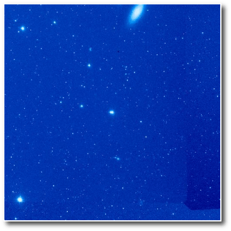
At the 100,000 light-year scale of the galactic disk, HD 80606, at ~190 light-years distance, is right next door. Its proper motion is currently shifting it across the sky at a rate of 1/75,000th of a degree per year, and it is receding from Earth at a rate of 1 light year per hundred thousand years (about 1/3 the rate of the Pioneer probes). As it drifts through space, our vantage of the system gradually changes. Right now, HD 80606 and its binary companion HD 80607 are centered in the 0.8 deg x 0.8 deg view just below. During the last ice age, they were out of the frame.

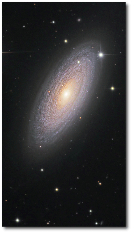
Upon receiving the above image from Goddard Skyview, I was surprised to see that HD80606 and HD80707 are currently less than a full-Moon’s width away from an impressive 10th-magnitude flocculent spiral galaxy. Turns out to be NGC 2841, which lies 46 million light years distant, contains over a billion transiting planets, and looks fantastic in this close-up, taken from Johannes Schedler’s backyard observatory:

Image: Panther Observatory Styria, Austria

This galaxy has also been imaged with Spitzer at 3.5 (blue), 4.5 (green) and 8 (red) microns. Warm dust heated by star formation in the arms glows falsely in the red. Star formation has all but shut off in the inner spheroidal region, which shines in the shorter-wavelength infrared light of an older spheroid stellar population.

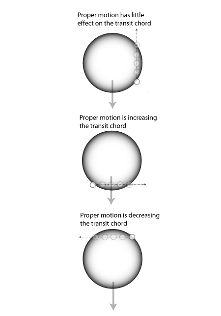
Where transiting planets are concerned, however, it’s quality, not quantity that matters, and proximity is everything. As our line of sight to the HD 80606 system slowly changes, the transit geometry will shift. While we know almost everything about HD 80606b’s orbit, the one thing that we don’t know is the orientation of the transit chord relative to the cardinal directions in the plane of the sky. As a result, the change in our viewpoint created by proper motion could be leading to a transit impact parameter that is either increasing, decreasing, or staying roughly the same.

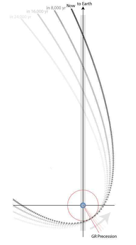
In the event that the proper motion were leading to the maximum increase in the impact parameter, and if the orbital orientation was fixed in space, then the transits could end as soon as 27,000 years from now. The orbit, however, is not fixed. Both the node and the periastron line are precessing as a result of rotational and tidal deformation in the star and the planet, as a consequence of the torque exerted by HD 80607, and as a result of general relativity. It turns out that the relativistic precession dominates, and is forcing ‘606b’s periastron to circulate with a period of about 600,000 years. The precession is prograde, and so as a result, the star-planet distance at the transit midpoint is currently decreasing by about 300 km every transit.

As a result, even for the least optimistic geometry, transits of HD 80606b will persist for roughly the next million years due to the commensurability between the time-scale for relativistic precession and the time for the line-of-sight inclination change to fully sweep the transit chord across the star. In addition, with careful (JWST-caliber) timing of the changing interval between the secondary eclipse and the primary transit, as well as the duration of the primary transit, one should be able to get both a test of general relativity and a constraint on the plane-of-the-sky rotational orientation of the system. Cool!

N-gram

There are a lot of good books in the public domain. In Oscar Wilde’s Picture of Dorian Gray, I’ve always been intrigued by the description of…

the yellow book that Lord Henry had sent him. What was it, he wondered. He went towards the little pearl-coloured octagonal stand, that had always looked to him like the work of some strange Egyptian bees that wrought in silver, and taking up the volume, flung himself into an armchair, and began to turn over the leaves. After a few minutes he became absorbed. It was the strangest book that he had ever read.  […] The style in which it was written was that curious jewelled style, vivid and obscure at once, full of argot and of archaisms, of technical expressions and of elaborate paraphrases […] There were in it metaphors as monstrous as orchids, and as subtle in colour.

Google books, with its vast digitized sea, imbues the esoteric with the convenience of a TV dinner. While sitting at the gate in O’Hare waiting for the flights that would take me to the Torun Conference a few years ago, it occurred to me that it might be cool if my talk had a scan from an original edition of De revolutionibus orbium coelestium. A minute later, it had been pulled from the ether by my computer.

(A Rebours makes decidedly better reading. While Copernicus’ great work is at once, full of argot, archaisms, and technical expressions, it is wholly devoid of metaphors as monstrous as orchids, and as subtle in colour.)

With millions of digitized books, one can step away from trying to find those individual bits of half-remembered ephemera, and instead treat all the words in all the books statistically. There was an article in Science last week (Michel et al. 2010) which received lots of press, and which contains a link to Google’s Ngram viewer.

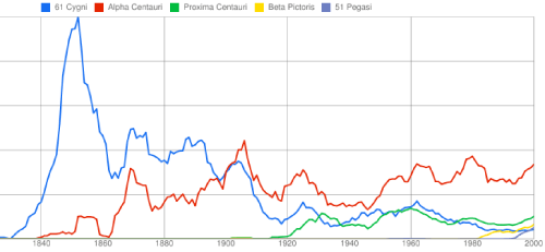
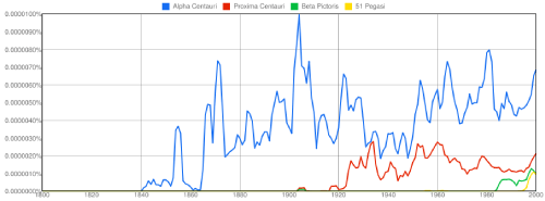
An “Ngram” is a neologism for a specific string of N words. The idea is that you can trace cultural trends by charting the frequency with which words appear in books. For example, for 5 million books published between 1800 and 2000, the frequencies of appearance of 61 Cygni, Alpha Centauri, Proxima Centauri, Beta Pictoris, and 51 Pegasi are:

61 Cygni, which, in 1838 was the first star to have its distance correctly measured, was a marquee attraction during the Nineteenth Century. As a result of Thomas Henderson’s timidity in publishing his parallax, it took Alpha Centauri, which is closer, brighter, and more alluring, more than 80 years to surpass 61 Cygni’s fame. Proxima, which was discovered in 1915, has never managed to be as popular as Alpha, and, until recent decades, has struggled to keep up with 61 Cygni. Beta Pictoris makes its debut in 1983, and 51 Pegasi starts turning up after 1995.

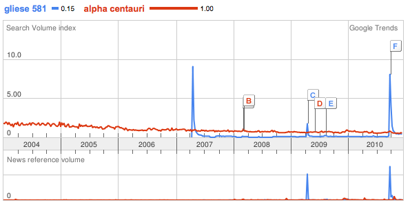
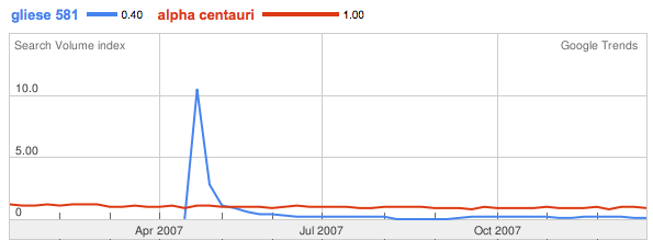
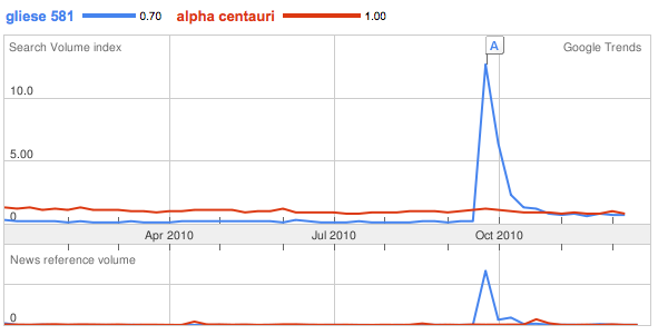
As a visit to Borders will quickly confirm, books are fast losing their status as a cultural linchpin. For topics of current interest, Google trends is more the destination of choice. Here, one can follow the share of the total global search volume that a particular N-gram elicits. News reference volume is also charted. Among the stars of interest, there is a steady stream of searches on Alpha Centauri. Against this background, there are three rather notable spikes associated with Gliese 581, which, prior to 2007, languished in complete obscurity.

After the 2007 spike, Gliese 581’s mojo quickly faded to a small fraction of Alpha Centauri’s.

Interestingly, though, the 2010 pattern is behaving differently. In the months following the most recent spike, Gliese 581 has been running neck and neck with Alpha C in competition for the world’s notice.

Shaken not stirred

Photo credit: Bill Lowenburg — From the Crash Burn Love Project

I sure enjoyed that article on Figure-Eight racing in last Sunday’s New York Times. The piece is a shameless sop, of course, to the smug ironic-hipster segment of the NYT readership — not unlike twelve-packs of Pabst Blue Ribbon stacked up in front of the checkout counter at Whole Foods — but it’s also a great story. The racers adhere to a pure recession-era hellenic ideal, risking life and limb for glory, complete with six-time world champion Bob Dossey channeling a latter-day wrath of Achilles.

And the exoplanet connection? Orbital mean-motion resonances with large libration widths bring to mind a smoothly-running Figure-Eight race. The planets roar around the parent star, continually missing each other at the intersections of their crossing orbits. Here’s an animation of the HD 128311 2:1 resonant pair, strobed over several hundred orbits.

(Animation was causing the site to slow down, so I took it down.)

To date, several such systems are known. In addition to HD 128311 b and c, a similar state of affairs also seems to hold in the HD 82943 and HD 73526 systems, both of which appear to harbor planets in 2:1 mean motion resonance with large libration widths. For all three of these systems, however, the degree of confidence that the correct dynamical configuration has been identified is somewhat less-than-satisfying. Rather than directly observing the resonant dynamics, one notes in each case that a whole bundle of model systems can be constructed which fit the radial velocity data. Within these large sets of allowed configurations, the ones that are dynamically stable over time scales of order the stellar lifetime tend to have large libration widths.

By contrast, Gliese 876 — the one system for which the radial velocity solution provides direct and unambiguous access to the resonant configuration — has its two largest planets lying very deeply in 2:1 resonance, and the libration width is just a few degrees. It bothers me that Gliese 876 seems to be so qualitatively different. It’s easy to wonder whether there might be an error of interpretation for the indirectly characterized systems.

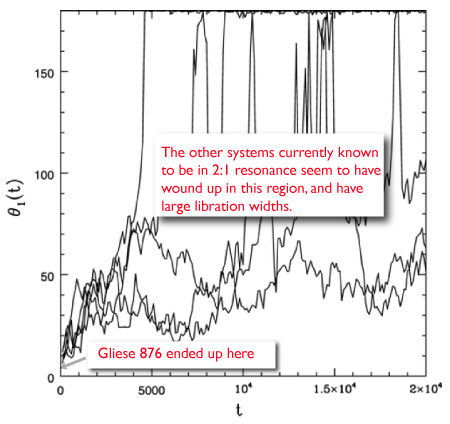
Resonance libration widths are more than just a curiosity. They provide a record of the conditions that likely existed in the protostellar disks from which the planets formed. A turbulent disk produces transient density fluctuations that cause the libration width of a resonant pair of planets to undergo a random walk, much as a stochastically driven pendulum will, on average, tend to gradually increase the height of its swing. The plot below (which comes from a 2008 ApJ paper written with Fred Adams and Anthony Bloch) shows the results of five individual simulations in which gravitational perturbations mimicking those arising from disk turbulence are applied to integrations of the Gliese 876 A-b-c system. In each case, the libration width of the resonant argument tends to increase with time. Perhaps the Gliese 876 system was very lucky, and despite being buffeted managed to end up with a tiny swing. More likely, the gas flow in Gliese 876’s disk was relatively calm and laminar.

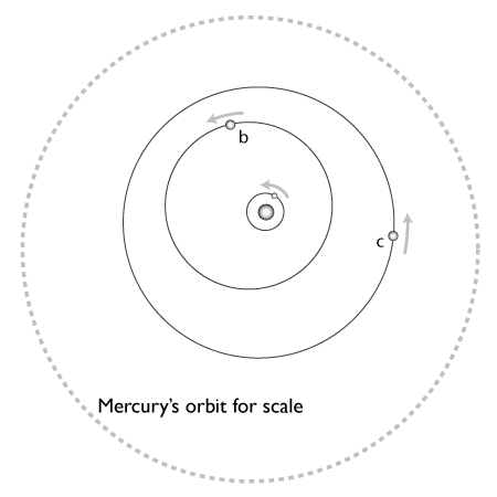
Until now, almost everything we know about extrasolar planets in resonance has come from the radial velocity surveys. This year, Kepler is also starting to contribute, with the announcement of  a new system — Kepler 9 — which exhibits detectable transit timing variations. The planets orbiting Kepler 9 were announced with media fanfare during the recent Haute Provence meeting, and a detailed article (Holman et al. 2010) will soon be published in Science. The Kepler 9 set-up is oddly reminiscent of Gliese 876. Two Saturn-sized (and somewhat less than Saturn-mass) planets orbit with periods currently in the vicinity of 19 and 39 days. Further in, an unfortunate super-Earth is stuck is a blistering 1.6-day orbit. Here are the orbits drawn to scale.

The planetary and stellar radii are not to scale, but rather, are sized to conform to the NASA press release artist’s impression of the system…

Kepler 9’s orbital geometry represents quite an extraordinary draw! All three planets can be observed in transit, and the strong gravitational interactions between the two outer planets lead to large deviations from strict periodicity. Indeed, the system is simultaneously tantalizing and maddening. The parent star is many times fainter than Gliese 876, meaning that it will be difficult to get a large collection of high-quality radial velocity measurements. In order to really characterize the dynamics of the system, it will be necessary to lean hard on transit timing measurements. The observations published in the Science article have a low per-point timing cadence; skilled amateur observers can obtain timing measurements that have higher precision and which significantly extend the time baseline, and so the system presents an excellent opportunity for small telescopes to obtain cutting-edge results. The parent star (in Lyra) is still up in the Northern Hemisphere’s evening sky, and there are transits coming up!

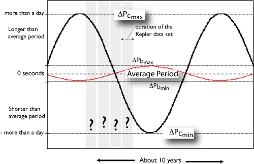
During the time that Kepler monitored the system last year, the orbit of the outer planet, “c” (P~38.9 d) was observed to be steadily decreasing by 39 minutes per orbit, and the orbital period of the inner planet, “b”  (P~19.2 d) was increasing by 4 minutes per orbit. Clearly, this state of affairs can’t continue indefinitely. If the system is in a 2:1 mean motion resonance, then over the long term, the periods of the two planets will oscillate around well-defined average values. The Kepler measurements strobed the system over a relatively small fraction of its overall cycle. An analysis of the planetary disturbing function (in which all but the most significant terms get thrown out) indicates that the libration time should be of order the orbital timescale (40 days) multiplied by the square root of the planets-to-star mass ratio (~100), or about ten years.

We don’t know exactly which part of the cycle Kepler dropped in on, and so the second derivative (rate of change of the rate of change) of the period could be either positive or negative. This means that there is a significant uncertainty on when the next transits will occur, but it also means that accurate measurements will immediately give a much better idea of what is going on.

The next opportunities will occur on October 5th (for 9c) and October 8th (for 9b). As always, observers should use the TRESCA website to double-check observing details and to submit light curves after the observations have been made. As the dates approach, I’ll post specific details for small-telescope observers — it will take a global effort to ensure that definitive observations are made. We’ll also soon be releasing an updated version of the systemic console that will allow for the modeling of TTVs in double-transit systems.

Extrapolations…

…are often risky, but can be illuminating nonetheless.

The astronomy decadal report, which was issued a few weeks ago, set forth three big-picture goals for the next decade: (1) searching for the first stars, galaxies, and black holes; (2) seeking nearby habitable planets; and (3) advancing understanding of the fundamental physics of the universe.

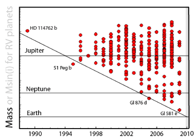
It’s looking quite likely that goal number two will be the first to get substantially met. For quite a while now, a plot of year of discovery vs. the known planetary Msin(i)’s has provided grist for speculation that the first announcement of an Earthlike Msin(i) will occur this year…

In all likelihood, the surface of the first Earth-mass object detected in orbit around a sun-like star will be better suited to oven-cleaning than life as we know it. An interesting question, then, is: when will the first potentially habitable planet be detected? As readers know, such a world will very likely be detected via either transit (MEarth, Warm Spitzer or Kepler) or by the radial velocity technique (HD 40307, Alpha Cen B, etc. etc.).

Earlier this year, I struck up an e-mail conversation with Sam Arbesman, a Research Fellow at Harvard who studies computational approaches to the social sciences. Sam has a rather eclectic spectrum of interests, and writes pieces for the Boston Globe and the New York Times on topics ranging from mesofacts to baseball statistics. He’s also in charge of collecting fares for the Milky Way Transit Authority.

We carried out a scientometric analysis to arrive at what we believe is likely to be a reasonably accurate prediction of the discovery date of the first potentially habitable extrasolar planet with a mass similar to Earth.

Our paper has been accepted by the journal PLoS One, and Sam just posted to arXiv, apparently with little time to spare. The best-guess date that emerged from the analysis is May 2011.

Audaciously, alarmingly close! Certainly soon enough, in any case, for us to look rather sheepish if we’re off by a significant amount…

Macrobes

Exciting times for the exoplanet field. The announcement of the first million-plus dollar world is only days to weeks to months or at most a year or two away, and in the interim, the planet census keeps expanding.

At the same time, however, all the new planets are accompanied by a certain creeping degree of frustration. I have a feeling that these worlds, and especially the super-Earths, will prove to be even more alien than is generally supposed. Artist impressions do a good job when it comes to gray and airless cratered surfaces, but are necessarily inaccurate or impoverished or both in the presence of masses more than a few tenths that of Earth. And because of the distances involved, we won’t be getting the really satisfying images any time soon.

With my provincial day-to-day focus on Gl 876, Gl 581, HD 80606 et al., I tend to forget that we’ve got a full-blown planetary system right here in our back yard. It caught me by surprise, months after the fact, and via a thoroughly tangential channel, that a sober-minded case can be made for the presence of methane-based life on Titan. In fact, a detailed case has been made, complete with specific predictions, and, startlingly, those predictions now seem to have been confirmed.

In 2005, Chris McKay (whose office was just down the hall when I worked at NASA Ames’ Planetary System Branch) wrote an Icarus paper with Heather Smith proposing that methanogenic life might be widespread on Titan. McKay and Smith argue that one macroscopic consequence of such life would be a depletion of ethane, acetylene, and molecular hydrogen in Titan’s near-surface environment. Recent work seems to indicate that all three compounds are indeed depleted, which is very interesting indeed.

The details, and an assessment of the odds are a topic for another post. The simple fact that Titan is in the running at all is absolutely remarkable. Toto, I’ve a feeling we’re not on Mars anymore. Methane-based life in the Saturnian system would seemingly stand a far higher chance of stemming from a completely independent genesis. If Titan has managed to put together a biosphere, then there could very well be more life-bearing planets in the Galaxy than there are people.

The prospect of widespread life on Titan brings to mind the descent of the Huygens probe on January 14, 2005. I remember wondering, in the days running up to the landing, what the probe was going to see, and thinking that it was a once-in-a-lifetime moment of anticipation. Titan is the only world in our Solar System in which there was seemingly a chance, albeit very slim, of having a genuinely world-altering scene unfold upon touchdown. I knew that in all likelihood, the scene was likely going to look something like a cross between the Viking  and Venera panoramas, but I couldn’t quite squelch that lotto-player’s like expectation that pictures of a frigid silurian jungle would be radioed back across light hours of space…
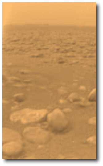
As everyone knows, there was no golden ticket in the chocolate bar, but might we still have a chance to see something really exotic when the next probe touches down?

It’s always seemed to me that the relatively mundane ground-level view at the Huygen’s landing site was somewhat at odds with the electrifyling promise implicit in the probe’s descent sequence. From 150 kilometers up, the haze is just starting to part — the view is not unlike the one that Percival Lowell had through his telescope of Mars. Faint dusky markings that one can connect in the mind’s eye to just about anything:
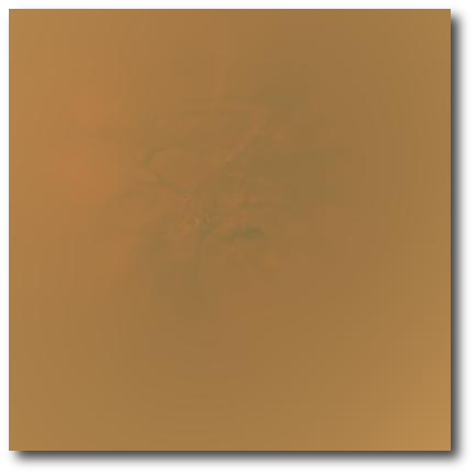
From 20 kilometers up, a wealth of detail is visible. Alien rivers, shorelines, islands?
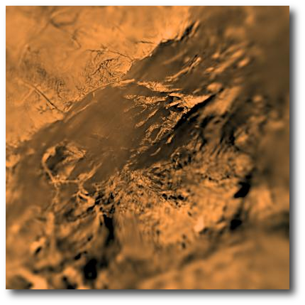
The Huygen’s signal was extremely weak. The images arrived in a jumble, with Earth’s largest radio telescopes straining to hear them. It’s interesting to imagine what the level of anticipation might have reached had we known of the atmospheric depletions, and had the images arrived in real time as the probe drifted down toward the surface. Here’s the view from six kilometers up. Think of the looking out the window of a Jetliner several minutes after the start of descent from cruising altitude:
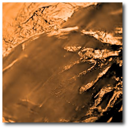
From 2 kilometers up:
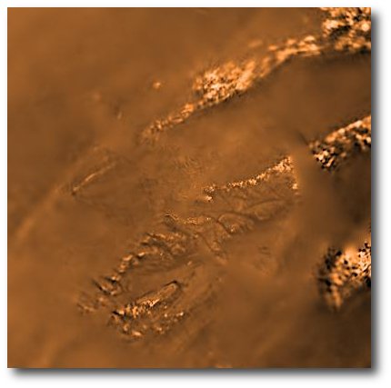
From .6 kilometers up:
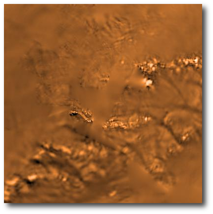
From a mere 200 meters altitude:
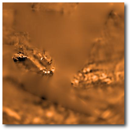
What if we carry out the same exercise and land a probe at a random spot on Earth? To roughly 1-sigma confidence, we’d come in for a splashdown somewhere in the ocean. Out of sight of land, no macroscopic life visible, just water, clouds and blue sky, and just like Huygen’s landing on Titan, a disappointment with respect to what might have been…

So I decided to wrap up the post by forcing the hand of chance. Using true random numbers (generated, appropriately enough by random.org through the use of Earth’s own atmospheric noise) I drew a single random location on the surface of a sphere, and calculated the corresponding longitude and latitude. The result?

-26.478972 S, 132.022361 E.

Google Maps makes it possible to drift in like Huygens for a landing sequence at any spot on Earth. The big picture, of course, is completely familiar, so the suspense is heightened in this case by successively zooming out.
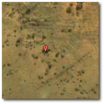
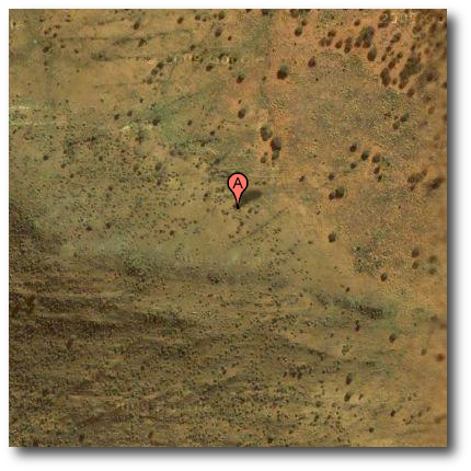
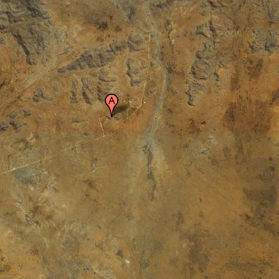
The next scene, which is roughly a mile on a side, is quite readily set into the mental context. The random spot is in the Australian outback. Red dust, scattered rocks, scrub brush, spindly trees, and most evocatively, a building, a cul-de-sac, and a lonely stretch of dirt road bisecting the lower right corner of the view. Of course, had the probe come in a few decades ago, the scene would be no less tantalizing than what we had from Huygens at similar altitude. Those could easily be boulders, not treetops.
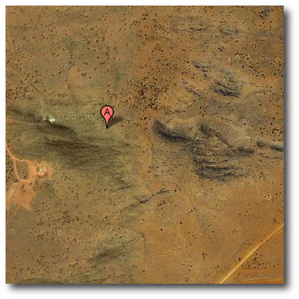
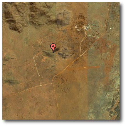
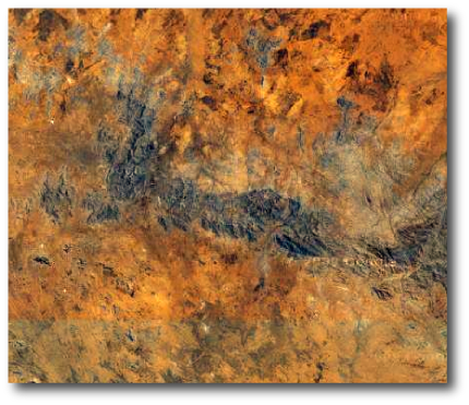
Aside from the roads, at a scale similar to where Titan was first revealed, Titan holds out, if anything, more promise than -26.478972 S, 132.022361 E:
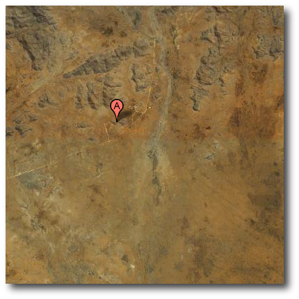

To set context, one can zoom all the way out. By coincidence, -26.478972 S, 132.022361 E is not far from the zone peppered by the reentry of Skylab on 11 July 1979, which ranged from 31° to 34°S and 122° to 126°E.

With a simulated Earth landing, we’re allowed to cheat, and get the full scoop on our landing spot. This is as simple as enabling geo-tagged photos and Wikipedia entries:
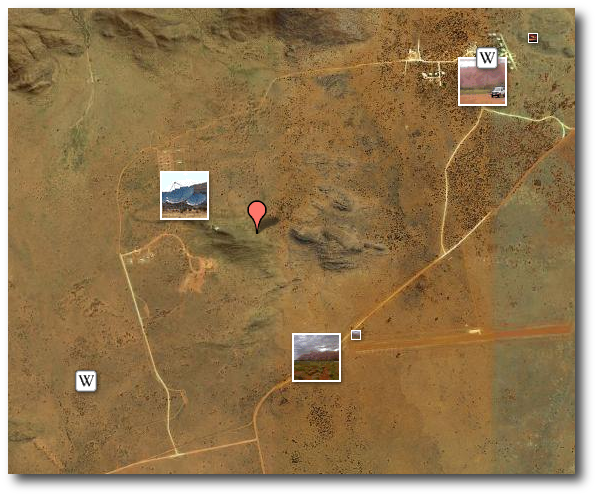
The wikipedia links are here and here. -26.478972 S, 132.022361 E is just over a rise from a solar power station on the Anangu Pitjantjatjara Yankunytjatjara local government area.

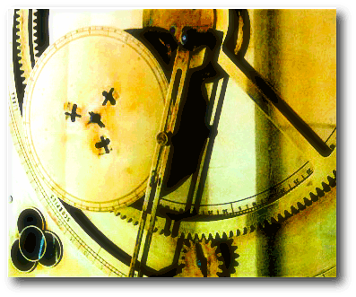
And imagine a probe touching down just in time to record this scene:

Image source.
Radius Anomalies

The radii of the transiting extrasolar planets have been the source of a lot of consternation. It’s very hard to tell the mass of a planet simply by looking at how large it is.

In our own solar system, there’s a well-delineated correlation between planetary size and planetary mass, with the only modest exception being Uranus and Neptune. Uranus has the larger radius and Neptune has the larger mass. With the extrasolar planets, on the other hand, the situation is notoriously less clear-cut. Transiting planets, with HD 209458b providing the textbook example, are often considerably larger than expected, hinting at a cryptic energy source.
With the WASP and the HAT surveys firing on all cylinders, the catalog of well-categorized transiting planets has been growing quite rapidly. There are now close to 90 planets with reasonably well determined masses and radii, so I thought it’d be interesting to take stock of the catalog with an eye toward evaluating how bad the radius problem really is.

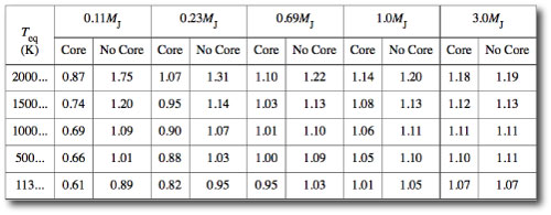
Back in 2003, Peter Bodenheimer and Doug Lin and I did a series of planet evolution calculations which solved for the equilibrium radii of giant planets made from hydrogen and helium (and both with and without solid cores). Our models spanned a range of planetary masses and surface temperatures, and they provide a baseline expectation for how large gas giant planets “should” be (radii are in Jovian units):

Clear trends can be seen by studying the table. For example, once planets get significantly more massive than Jupiter, they stop increasing their radii. This is a consequence of the interior equation of state growing progressively more electron degenerate. It’s also true that the hotter a planet gets, the larger it’s expected to be, and a core of heavy elements causes a planet to have a smaller overall radius.

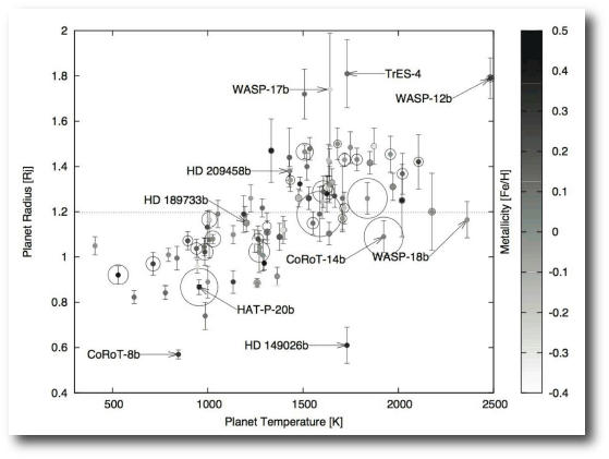
With the baseline “no core” models in hand, it’s straightforward to see whether a newly discovered planet conforms to expectations. With some exceptions, the extrasolar planets have not tended to conform to expectations (a state of affairs that has held up quite robustly, in fact, across the entire exoplanet field, where theoretical predictions have rarely presented any real utility). A significant fraction of hot Jupiters are a lot larger than expected, and there are also some that have turned out to be considerably smaller than expected. For a given planet, we can define the “radius anomaly” as the fractional discrepancy between the predicted radius and the observed radius. A planet like HD 209458b has a large positive radius anomaly, whereas a planet like HD 149026b has a large negative radius anomaly.

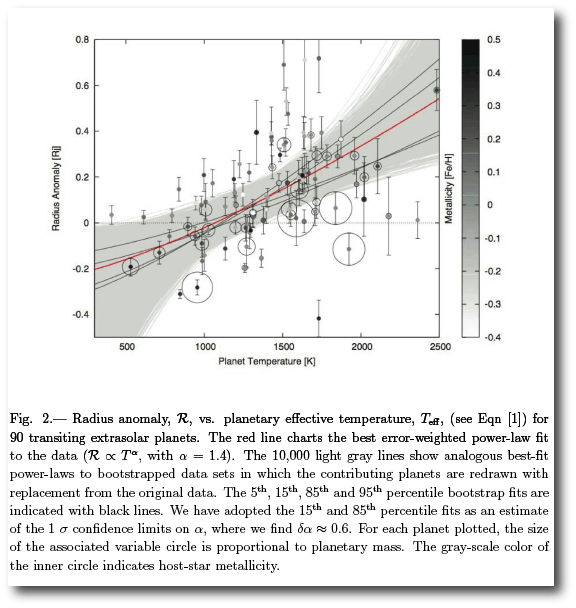
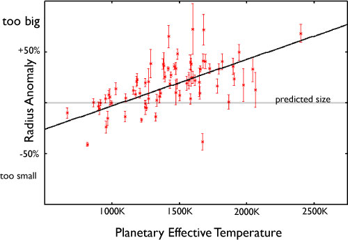
One can garner clues to the source of the radius problem for extrasolar planets by regressing the radius anomalies against possible explanatory variables. The most dramatic effect comes when one plots radius anomaly as a function of effective planetary surface temperature:

As a general rule, the hotter the planet, the more severe the radius anomaly. This points to ohmic heating as the most likely culprit for pumping planets up. The hotter the planet gets, the larger the ionization fraction in the atmosphere, and the more effectively the weather is able to act as a toaster. Konstantin Batygin and Dave Stevenson’s recent paper on this topic is almost certainly barking up the right tree.

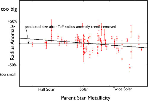
Another interesting correlation arises when one plots radius anomaly versus stellar metallicity after removing the planet temperature trend observed in the plot above. In this case, there’s a modest correlation with the opposite sign:

Planets with negative radius anomalies tend to orbit metal rich stars. This is a natural (and expected) consequence of the core accretion hypothesis for giant planet formation.

Simple linear dependencies on planetary temperature and stellar metallicity are able to account for more than half (but not all) of the observed variance in the radius anomalies. The missing factor could come from a number of sources — nonlinearity in the correct model description, observational biases, or perhaps something else altogether…

Finally, in the this-just-in Department, there’s a paper up on astro-ph this week detailing the discovery of HAT-P-18, and and HAT-P-19. These two planets certainly don’t enhance the suggestiveness of the above plots — their anomalies are anomalous. Both of the new Hats are relatively cool, relatively low mass planets orbiting relatively metal rich stars. And they’re both swelled up! Tidal heating? Could be.

A second Laplace resonance

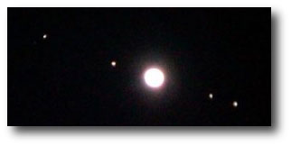
It’s no exaggeration to assert that Galileo’s unveiling of Io, Europa, Ganymede and Callisto counts among the epic scientific discoveries of all time.

And certainly, it’s fair to say that the Galilean satellites of Jupiter constitute the original exoplanetary system. The Galilean satellites have been producing scientific insights for over four hundred years. Nearly all of the modern exoplanetary discoveries have antecedents — some quite recent, some centuries old — in Jupiter’s four moons.

The Galilean satellites can all be observed in transit across the face of Jupiter, and as early as 1656, the Sicilian astronomer Giovanni Hodierna, with his Medicaeorum Ephemerides, emphasized the importance of transit timing measurements for working out accurate predictive tables. In the late 1660’s, University of Bologna Professor Giovanni Cassini’s timing measurements and associated tables for the Jovian system were so impressive that he was tapped by Jean-Baptiste Colbert and Louis XIV to become director of the newly established Paris Observatory.

Giovanni Domenico Cassini (1625-1712). Prior to holding the directorship of the Paris Observatory, he was the highest paid astronomer at the University of Bologna, having been appointed to his professorship by the Pope.

Throughout the 1670s and 80s, Cassini wrestled with the fact that accurate transit timing measurements for the Jovian satellites create serious difficulties for models in which the moons travel on fixed orbits. Irregularities in the transit timings made from the Paris Observatory led to Ole Roemer’s determination of the finite speed of light in 1676, and by the early 1700s, observations of transit duration variations revealed that rapid nodal precession occurs in the Jovian system.

By middle of the Eighteenth Century, adequate data were in hand to demonstrate that a very curious relationship exists between the orbits of Io, Europa, and Ganymede. In 1743, the Swedish astronomer Pehr Wilhelm Wargentin (the first director of the Stockholm Observatory) published tables which made it clear that the 1:2:4 ratio in periods between Ganymede, Europa and Io is uncannily exact. Wargentin’s tables implied that a triple eclipse (in which all three satellites transit at once) would not occur until 1,319,643 CE at the earliest, and that the “argument”

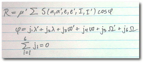
between the mean longitudes of the satellite orbits is maintained to an extraordinary degree of accuracy. Geometrically, this means that the satellites engage in a cycle of six successive moon-moon conjunctions during the course of one Ganymedian orbit, and in so doing, manage to continually maintain ?L=180°:

Laplace realized that a dynamical mechanism must be responsible for maintaining the cycle of conjunctions, and in 1784, was able to show that the angle ? is subject to a pendulum-like oscillation. If the satellites are perturbed slightly, then over the time, the satellite-satellite interactions conspire to cause ? to oscillate, or librate, back and forth about the equilibrium value of 180°. His theory for the satellites allowed him to derive the masses of the moons, and also predicted that the oscillation period for ? would be 2270d 18h.

In Laplace’s time, the observations were not accurate enough to sense any measurable amplitude for the libration — it appeared that the satellites were perfectly placed in the 1:2:4 resonant condition. We now know, however that ? librates with a tiny amplitude of 0.064°, and that the period of oscillation is 2071d, quite close to the value predicted by Laplace. Yoder and Peale (1981) have shown that the highly damped libration of ? can be understood as arising from a near-balance between tidal dissipation in Jupiter and tidal dissipation in Io. The presence of a dissipative mechanism has allowed the marble to have settled almost precisely into the bottom of the bowl.

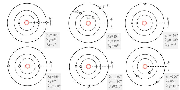
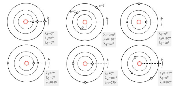
On this evening’s astro-ph mailing, our team has posted a paper that describes our discovery of a second example of a Laplace three-body resonance. Continued radial velocity monitoring of the nearby red dwarf star Gliese 876 has shown that the well-known P~30d and P~61d giant planets in the system are accompanied by an additional planet with a mass close to that of Uranus and an orbital period P~124d. In contrast to the Jovian system, the best fit to the observations shows that the Laplace relation is librating around ?=0°, and that triple conjunctions do occur. The diagram above is easily modified to convey the schematic geometry of the new system:

The actual state of affairs, however, is more complicated than shown in the above diagram. The total mass of planets in the Gliese 876 system is about 1% the mass of the central body, whereas Jupiter is roughly 5000 times more massive than its satellite system. This means that the Gliese 876 planets experience proportionally larger mutual gravitational interactions than do the Galilean satellites. In addition, the orbits are much more eccentric, and the planet-planet secular interaction causes a rapid precession of 14° per orbit of the outer planet. We can, however, plot the orbits in a co-precessing frame in order to view the cycle at four equal time intervals:

The libration of the Laplace argument, ?, around zero has an amplitude of ~40°, indicating that the GJ 876 “pendulum” packs a swing that’s 625 times larger than that of the Galilean satellites. Indeed, when the system configuration is integrated forward in time for hundreds of years, it’s clear that a simple pendulum equation is not able to describe the evolution of the Laplace angle. The oscillations are chaotic, with a Lyapunov time measured in a mere hundreds to thousands of years, and the theory, especially if there is a non-coplanar component to the motion, will require Laplace-level expertise in the use of the disturbing function…

There’s more… stay tuned for the next post.

That other angle

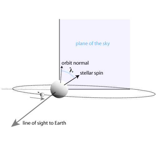
Some of the biggest exoplanet news so far this year has arrived in the form of Rossiter-McLaughlin measurements of the sky-projected misalignment angles, λ, between the orbital angular momentum vectors of transiting planets and their stellar spin vectors.

A significantly non-zero value for λ indicates that a system was subject to some rough action in the distant past. Both planet-planet scattering and Kozai migration, for example, can lead to systems with non-negligible λ’s. The recent paper by Triaud et al. (covered here) showed that such processes may be responsible for a startlingly significant fraction of the known transiting-planet systems.

The angle λ has the advantage of being measurable, but it has marked disadvantage of informing us only of the projected geometry of the system. To get a sense of the physically relevant quantity — the true degree of spin-orbit misalignment — one needs the direction of the stellar spin vector.

Kevin Schlaufman, one of the graduate students in our program here at UCSC, has worked out a very clever method of getting a proper statistically supportable guess of the complement misalignment angle between the orbit of the plant and the spin of its host star along the line of sight. I have to say that I’m quite enthusiastic about Kevin’s paper — it’s a big jump, not an incremental advance, and it’s well worth reading.

The method leverages the fact that a mature main-sequence star of given mass and age has a fairly predictable rotation period. Sun-like stars form with a wide range of rotation periods, but by the time they reach an age of ~0.5 billion years, there is a reasonably well-defined rotational period-stellar mass relation. During the remainder of their lives, main sequence stars then slow their rotation by shedding angular momentum via Alfven-like disturbances. Stellar spin-down rates are relatively large early on, and decrease with the passage of time.

A star’s projected rotational velocity can be measured by looking at the amount of rotational broadening in the spectral lines. This gives V_rot*sin(i_s), where i_s is the unknown angle between the star’s spin pole and the line of sight. The essence of the Schlaufman method is then immediately apparent. The mass and the age of the star allow you to infer V_rot. You measure V_rot*sin(i_s), and then bam! The inclination angle, i_s, is determined.

Reality, of course, is not so clear-cut. One has a host of errors and intrinsic variation to deal with, all of which blur out one’s ability to precisely determine i_s. Nevertheless, Kevin shows quite convincingly that the method has utility, and that it is possible to identify transit-bearing stars that are very likely strongly misaligned with the plane of the sky.

The results of the analysis confirm that massive and eccentric transiting planets (such as oklo.org fave HD 17156b) are substantially more likely to have significant spin-orbit misalignment than are garden variety Jupiter-mass hot Jupiters on circular orbits. Furthermore, to high confidence, it seems that systems with substantial spin-orbit misalignment tend to have host stars with masses greater than 1.2 solar masses. A reasonable conclusion is that there are two distinct and productive channels for generating short-period giant planets. The first is a disk migration process that leaves everything calm, orderly and aligned. The second, most likely involving Kozai cycling or a variant thereof, is telegenic, action packed, and leaves a system confused and misaligned, and perhaps stripped of several original fellow planets.

312 candidates

It’s not often that a near-doubling of the planetary census arrives in one chunk, and so the paper detailing the latest Kepler results is of quite extraordinary interest.

It’s definitely going to be tricky to use the results in the Kepler paper to draw secure new conclusions about the true underlying distribution of planets. Nevertheless, the results look quite intriguing from the standpoint of back-of-the-envelope speculations.

Details: the paper contains a list of 312 candidate planets originating from 306 separate stars. A further 400 stars with candidate planets have been held back (see yesterday’s post), largely because they are either bright enough for high-quality Doppler follow-up at less-than-exorbitant cost, or harbor candidates with radii less than 1.5 that of Earth, or both. The paper states that the 312 candidate planets were primarily culled from an aggregate of 88,196 target stars dimmer than magnitude 14. The analysis is based on two blocks of photometry, one lasting 9.7 days (starting on May 2 2009) and one lasting 33.5 days (starting on May 13 2009).

The candidates have a slightly eclectic selection of associated data. The main table lists a radius, a transit epoch, and an orbital period for each candidate. There’s information about the parent stars as well, including apparent magnitude, effective temperate, surface gravity, and stellar radius. This is enough to make some intriguing plots. For example, the splash image for this post is a Hertzsprung-Russell diagram charting the locations of the candidates’ parent stars. The sizes of the points are directly proportional to the planet radii, and the color code is keyed to estimated planetary effective temperature. Most of the planets have surface temperatures of order 1000K or more, but there’s one rather singular object in the list, a 1.34 Rjup candidate on a 10389.109(!)-day orbit about a 9.058 solar radius G-type giant that (if it’s a planet) would have a photospheric temperature of order 180K. Certainly, a 1.34 Rjup radius is intriguing for such an object, as any non-pathological cold giant planet should be the size of Jupiter or smaller. Presumably, if the light curve showed evidence of a Saturn-style ring system, or better yet, an Earth-sized satellite, then KIC11465813 would chillin’ in the V.I.P. room.

A question of great interest is whether the list of candidates can add support to the recent radial velocity-based result that a large fraction of ordinary stars in the solar neighborhood are accompanied by a Neptune-or-lower mass planet with an orbital period of 50 days or less.

To get a first idea, I did the following quick (and extremely rough) Monte-Carlo calculation. I took 88,196 stars, and assumed that half of them have a planet with an orbital period drawn uniformly from the 1-d to 50-d orbital range. I then drew the planet masses uniformly from the 1-Earth-mass to 17-Earth-mass range, assumed Neptune-like densities of 1.6 gm/cc, circular orbits, and random orientations. For simplicity, the parent stars’ masses and radii are distributed uniformly from 0.7 to 1.3 times the solar value. I assumed that the 88,196 stars were observed continuously for 33.5 days, and require two transits to appear within the observation interval for a candidate to count. In keeping with the redaction policy, candidates are rejected if their radii were less than 1.5 that of Earth.

The simulation suggests that ~1100 candidate planets should be present in a 88,196 star sample. Encouragingly, this is at least order-of-magnitude agreement, although there’s a hint that the Kepler yield might be lower than what the RV results are implying. It will be very interesting to see what a more careful comparison has to say…

Intrigue

It’s always exciting when the exoplanets rise to the fore of the national discourse.

This morning’s New York Times has a very interesting article about the Kepler Mission’s proprietary data policy. In April, NASA granted the Kepler team an additional window, through February 2011, in which photometry for 400 particularly interesting stars is to be kept out of the public domain.

The article contains all the elements of exoplanetary intrigue that foreshadow traffic spikes for oklo.org in the months ahead. From the P.I., Bill Borucki:

“If I sent you 0’s and 1’s it would be useless… If we say ‘Yes, they are small planets — you can be sure they are.'”

From Ohio State’s Scott Gaudi:

“They need help,” he said, “If they were more open they would be able to get more science out…”

Delicious mention of formal non-disclosure agreements. Big-picture discussions of the meaning of data ownership in the context of federally funded research. 12,000 “suspicious dips” painstakingly distilled to 750 planetary candidates — a near-doubling, in one fell swoop, of the galactic planetary census.

And the oklo.org take? The astronomical enterprise is sometimes an excellent sandbox, a model, for understanding real-world problems. As an interested outsider, I definitely relish the challenges posed by a high-profile data set released under partial duress — a collection of both the ones and the zeroes, where the redactions can speak volumes.

The inverse problem

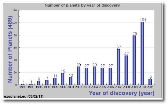
Transit timing variations have a certain allure. Most extrasolar planets are found by patiently visiting and revisiting a star, and the glamour has begun to drain from this enterprise. Inferring, on the other hand, the presence of an unknown body — a “Planet X” — from its subtle deranging influences on the orbit of another, already known, planet is a more cooly cerebral endeavor. Yet to date, the TTV technique has not achieved its promise. The planet census accumulates exclusively via tried and true methods. 455 ± 21 at last count.

Backing a planet out of the perturbations that it induces is an example of an inverse problem. The detection of Neptune in 1846 remains the classic example. In that now increasingly distant age where new planets were headline news, the successful solution of an inverse problem was a secure route to scientific (and material) fame. The first TTV-detected planet won’t generate a chaired position for its discoverer, but it will most certainly be a feather in a cap.

Where inverse problems are concerned, being lucky can be of equal or greater importance than being right. Both Adams’ and Le Verrier’s masses and semi-major axes for Neptune were badly off (Grant 1852). What counted, however, was the fact that they had Neptune’s September 1846 sky position almost exactly right. LeVerrier pinpointed Neptune to an angular distance of only 55 arc-minutes from its true position, that is, to the correct 1/15,600th patch of the entire sky

In the past five years, a literature has been growing in anticipation of the detection of transit timing variations. The first two important papers — this one by Eric Agol and collaborators, and this one by Matt Holman and Norm Murray — came out nearly simultaneously in 2005, and showed that the detection of TTVs will be eminently feasible when the right systems turn up. More recently, a series of articles led by David Nesvorny (here, here, and here) take a direct stab at outlining solution methods for the TTV inverse problem, and illustrate that the degeneracy of solutions, the fly in the ointment for pinpointing Neptune’s orbit, will also be a severe problem when it comes to pinning down the perturbers of transiting planets from transit timing variations alone.

In general, transit timing variations are much stronger and much easier to detect if the unseen perturbing body is in mean-motion resonance with the known transiting planet. In a paper recently submitted to the Astrophysical Journal, Dimitri Veras, Eric Ford and Matthew Payne have carried out a thorough survey of exactly what one can expect for different transiter-perturber configurations, with a focus on systems where the transiting planet is a standard-issue hot Jupiter and the exterior perturber has the mass of the Earth. They show that for systems lying near integer period ratios, tiny changes in the system initial conditions can have huge effects on the amplitude of the resulting TTVs. Here’s one of the key figures from their paper — a map of median TTVs arising from perturbing Earths with various orbital periods and eccentricities:

The crazy-colored detail — which Veras et al. describe as the “flames of resonance” — gives the quite accurate impression that definitive solutions to the TTV inverse problem will not be easy to achieve. One of the conclusions drawn by the Veras et al. paper is that even in favorable cases, one needs to have at least fifty well-measured transits if the perturber is to tracked down via timing measurements alone.

The Kepler Mission holds out the promise of systems in which TTVs will be simultaneously present, well measured, and abundant. In anticipation of real TTV data, Stefano Meschiari has worked hard to update the Systemic Console so that it can be used to get practical solutions to the inverse problem defined by a joint TTV-RV data set. An improved console that can solve the problem is available for download, and a paper describing the method is now on astro-ph. In short, the technique of simulated annealing seems to provide the best route to finding solutions.

A data set with TTVs alone makes for a purer inverse problem, but it looks like it’s going to be generally impractical to characterize a perturber on the basis of photometric data alone. Consider an example from our paper. We generated a fiducial TTV system by migrating a relatively hefty 10 Earth-mass planet deep into 2:1 resonance with a planet assumed to be a twin to HAT-P-7. We then created data sets spanning a full year, and consisting of 166 consecutive measurements, each having 17-second precision, and a relatively modest set of radial velocity measurements. We launched a number of simulated annealing experiments and allowed the parameters of the perturbing planet to float freely.

The resulting solutions to the synthetic data set cluster around configurations where the perturber is in 2:1 resonance (red symbols), and solutions where it is in 3:1 resonance (blue symbols). Furthermore, increasing the precision of the transit timing measurements to 4.3 seconds per transit (solid symbols) does little to break the degeneracy:

The upshot of our paper is that high-quality RV measurements will integral to full characterizations of the planets that generate TTVs. At risk of sounding like a broken record, this means that to extract genuine value, one needs the brightest available stars for transits…

de-aliased

It’d be rather unsettling to sit down with a cup of coffee one morning, and learn from astro-ph that the orbital period of Mars is not 1.88 years as is widely believed, but is rather a mere 7.83 months.

Last week, Rebekah Dawson and Dan Fabrycky posted a paper that gave me an equivalent jolt, and which has likely touched off a certain uproar within the planet-hunting community. Their claim is that the periods of a number of A-list planets, including 55 Cnc e and HD 156668 b are in fact aliases, and that the true periods of these worlds are startlingly different. Dawson and Fabrycky argue that the true period of 55 Cnc e is a fleet 0.7365 days (revised from 2.817d), and that HD 156668b orbits with a period of 1.2699 days rather than the published value of 4.6455d. Other well-known worlds may well be in line for a similar treatment.

Sometimes, things seem very clear in retrospect. In the graph just below, I’ve plotted the reflex velocity curves for two planets. One has a period of 1.61803 days, the other has a a period of 2.61803 days. If one happens to observe only at the times when the curves intersect, then it’s clear that there’s no way to tell them apart.

In the particular case above, the intersections of the sinusoids are separated by exactly one day. If the true period of the system is 1.61803 days, then we would say that the 2.61803 day period is an alias produced by the 1-day observing frequency. In general, for an observing frequency, f_o, and a true period, f_t, aliases exist at frequencies f=f_t+m*f_o, where m is an integer.

Aliases are a problem in Doppler surveys because observations are most efficiently done when the star is crossing the meridian, leading to a natural spacing of one sidereal day (23h 56m) between data points. Further periodicities in data-taking arise because RV survey time is usually granted during “bright” time when the Moon is up, and as a consequence of the yearly observing season for non-circumpolar stars. Aliases are minimized when observations are taken randomly, but the nuts and bolts of the celestial cycles impose regularity on the timestamps.

In reducing the period of 55 Cnc e to a sizzling 17.7 hours, the probability that the planet transits is raised to a very respectable 25%. Seems to me like rolling the dice with a few hours of Warm Spitzer time might be in order.

Habitable Worlds

Gough Island. Image Source.
Urbana, Illinois, the quintessential Midwestern University town, was a fine place to grow up, but it is sited in a landscape that is neither remote nor exotic.

Lifting up from Willard Airport just south of town, the near-absolute flatness of the landscape, planed by the last glacial advance, extends in a patchwork of corn and soybean fields to every horizon.


Something about the first-glance monotony of the Illinois landscape gradually instills a heightened sensitivity to the subtle detail inherent in a sense of place. Ray Bradbury, in Something Wicked This Way Comes, captures the essence of this perfectly. I think that living in Illinois also instilled a fascination with maps of the distant and rugged corners of the world.

I spent a lot of time poring over the maps that come with National Geographic. I’ve always been particularly drawn to the region corresponding roughly to the South Atlantic Anomaly, the vast expanse of the Southern Ocean that spans the temperate through subarctic latitudes. In the region roughly equidistant from South America, Africa and Antarctica, the maps show only a few specks of land: St. Helena, Tristan da Cunha, Gough, Bouvet. These islands, on the basis of their latitudes alone, seemed like they might be “habitable”, but the colossal scale imposed by millions of square miles of deep water, left them completely unresolved.

Within a few years, we’ll also know about extrasolar planets that just might be habitable. That is, we’ll have specific, concrete knowledge of worlds with radii and masses similar to Earth, on orbits within their parent star’s so-called habitable zones. But in all likelihood, for quite a while after that, a few spare, unadorned facts will constitute the bulk of our information about those planets — it’ll be left to extrapolation, to flights of conjecture and guesswork, to fill in the details.

The situation seems oddly parallel to the maps of the Southern Ocean. I can remember ranging over the names and coordinates of the the cryptic dots in the expanse of blue, and wondering, what are they like? There was nothing about Inaccessible I. in the public library. There was hardly a mention, of St. Helena I. (U.K.), other than a few maddeningly sketchy fragments in the Encyclopedia Britannica. Napoleon, after Waterloo, had been famously dispatched there, precisely because of its remoteness and isolation. Almanacs are invariably fond of listing the fact that Bouvet is the most isolated spot of land on Earth.

Like a current-day version of the TPF mission, the advent of Google and the Internet have brought the worlds of the Southern Ocean into focus.

Tristan da Cunha. Image Source.
Tristan da Cunha is dominated by a steep-sided 2000-meter volcano that last erupted in 1961. Two hundred and sixty people live on the island, making it the most isolated permanently inhabited spot on Earth. With Google, it’s possible to explore in great detail, although actually going there is not easy. There’s no airstrip. The only way in is by boat.

To get a better sense of scale, I superimposed the island on Urbana, Illinois, for a personalized juxtaposition of the exotic and the familiar.

Even more remote, is Gough Island. Until last year, it was hard to find good pictures of Gough. The views all seemed the same — a craggy heap of lava in the misty distance from the decks of ships. Recently, though, Google pointed me to an absolutely fantastic set of annotated photos, taken by Chantal Steyn, who spent an entire year during 2008-2009 on the island as part of an 8-person team that staffed a South African weather station on the Island. Suddenly, Gough comes spectacularly to life, the very picture of a habitable, yet alien world.

Mount Zeus on Gough Island. Image Source.

Further south, and far more formidable, is Bouvet. Nobody seems to be there, but oddly, the island has a top-level internet domain code (.bv) for which there are six registered hosts…

Image Source.
Paradigm upended?


Controversy generates revenue for exoplanet weblogs and supermarket tabloids alike, so I’m always happy when planet-related press releases roll out dramatic, far-reaching claims. Last week’s ESO press release — “Turning Planetary Theory Upside Down” — was quite satisfactory in this regard…

Upon digging into the back story, one finds that the observations underlying the press release are fully uncontroversial — it’s the big-picture interpretation that’s turning heads. Using Doppler velocity measurements taken during transit, Triaud et al. (preprint here) have measured the sky-projected misalignment angles, λ, for six of the transiting planets discovered by the SuperWASP consortium.

After an initial run of nine transiting planets were found to have sky-projected misalignment angles close to zero, the current count now has 8 out of 26 planets sporting significant misalignment. In the standard paradigm where hot Jupiters form beyond the ice line and migrate inward to reach weekend-length orbits, one would expect that essentially all transiting planets should be more or less aligned with the equators of their parent stars.

The standard migration paradigm, however, leaves at least two questions rather vaguely answered. First, why do the hot Jupiters tend to halt their inward migration just at the brink of disaster? The distribution of orbital periods — slew of selection biases aside — shows a durable peak near ~3 days. Second, why are transiting planets with well-characterized companions so scarce? In general, if one finds a giant planet with a period of ~10 days or more, the odds are excellent that there are further planets to be found in the system. For the known aggregate of transiting planets, and for hot Jupiters in general, additional planets with periods of a few hundred days or less are only infrequently found.

HD 80606b provides a clue that processes other than disk migration might be generating the observed population of hot Jupiters. The planet HD 80606b, its parent star HD 80606, and the binary companion HD 80607 form a “hierarchical triple” system, in which the two large stars provide an unchanging Keplerian orbit that drives the orbital and spin evolution of HD 80606b. If we imagine that HD 80606b and HD 80606 are both subject to small amounts of tidal dissipation, then to plausible approximation, this paper by Eggleton & Kiseleva-Eggleton argues that (i) the orbital evolution of “b”, (ii) the spin vector of “b”, and (iii) the spin vector of HD 80606 itself  can be described by a set of coupled first-order ordinary differential equations:

where e and h are vectors describing the planetary orbit, and where Ω_1 and Ω_2 are the spin vectors for HD 80606 and HD 80606b. The equations are somewhat more complicated than they appear at first glance, with expressions such as:

making up the various terms on the right hand sides.

Numerical integrations of the ODEs indicate that solutions exist in which the e and h vectors for `606b are bouncing like a ’64 Impala. Check out, for example, this solution vector animation by Dan Fabrycky (using initial conditions published by Wu and Murray 2003) which shows the leading scenario for how HD 80606b came to occupy its present state.
HD 80606b is imagined to have originally formed in a relatively circular orbit that was roughly 5 AU from its parent star, and which happened to be at nearly a right angle to the plane of the HD 80606-HD80607 binary orbit:

The large mutual inclination led to Kozai oscillations in which ‘606b was cyclically driven to very high eccentricity. During the high-eccentricity phases, tidal dissipation within the planet gradually drained energy from the orbit and decreased the semi-major axis:

Eventually, the orbital period became short enough so that general relativistic precession was fast enough to destroy the Kozai oscillations, and the planet was marooned on a high-eccentricity, gradually circularizing orbit that is severely misaligned with the stellar equator — exactly what is observed:

With HD 80606b, the case for Kozai-migration is pretty clear cut. The guilty party — the perturbing binary companion — is sitting right there in the field of view, and the scenario provides an easy explanation for anomalously high orbital orbital eccentricity. The only “just-so” provision is the requirement that the planet-forming protoplanetary disk of HD 80606 started out essentially perpendicular to the orbital plane of its wide binary companion.

The Triaud et al paper and the press release draw the much more dramatic conclusion that Kozai cycles with tidal friction could be the dominant channel for producing of the known hot Jupiters. From the abstract of their paper:

Conclusions. Most hot Jupiters are misaligned, with a large variety of spin-orbit angles. We observe that the histogram of projected obliquities matches closely the theoretical distributions of using Kozai cycles and tidal friction. If these observational facts are confirmed in the future, we may then conclude that most hot Jupiters are formed by this very mechanism without the need to use type I or II migration. At present, type I or II migration alone cannot explain the observations.

Can this really be the case? Might it be time to start reigning in the funding for studies of Type II migration in protostellar disks?

A key point to keep in mind is that Rossiter-McLaughlin measurements yield the sky-projected misalignment angle, λ, between the stellar spin and planetary orbital angular momentum vectors, and not the true misalignment angle, ψ, in three-dimensional space. That is, with transit spectroscopy alone, you can’t discern the difference between the following configurations:

In a paper published in 2007, Dan Fabrycky carried out integrations of the Eggleton-Kiseleva-Eggleton equations for an ensemble of a thousand star-planet-star systems that experience HD80606-style Kozai migration coupled with tidal friction. From the results of the integrations, he constructed a histogram showing the distribution of final misalignment angles, ψ:

The first nine Rossiter-McLaughlin observations of transiting planets all produced values for λ that were close to zero, in seeming conflict with Fabrycky’s distribution for ψ. The jump-the-gun conclusion, then, was that Kozai-migration is not an important formation channel for hot Jupiters.

With the spin-orbit determinations that appear in the Triaud et al. paper, there are now a total of 26 λ determinations. A fair fraction of the recent results indicate severely misaligned systems, and Triaud et al. show a histogram over λ (or in their notation, β):

In order to compare the observed distribution of λ measurements with Fabrycky’s predicted distribtion of Kozai-migration misalignments, ψ, Triaud et al. assume that the distribution of spin axes for the transit-bearing stars is isotropic. With this assumption, one can statistically deproject the λ distribution and recast it as a &#968 distribution, giving a startlingly good match between Fabrycky’s theory (blue dashed line) and observation:

When I first saw the above plot, I had a hard time believing it. The assumption that the spin axes of transit-bearing stars are isotropically distributed seems somewhat akin to baking a result into the data. Nevertheless, it is true that if Kozai migration produces the hot Jupiters, then the current ψ distribution is right in line with expectations.

In early 2009, Fabrycky and Winn did a very careful analysis of the 11 Rossiter measurements that were known at that time. Among those first 11 measurements, only XO-3 displayed a significant sky-projected spin-orbit misalignment. From the sparse data set, Fabrycky and Winn concluded that there were likely 2 separate populations of transit-bearing stars. One population, in which the spins and orbits are all aligned, constitutes (1-f)>64% of systems, whereas a second population, sporting random alignments, is responsible for f<36% of systems (to 95% confidence).

Bottom line conclusion? More Rossiter-McLaughlin measurements are needed, but I think its safe to say that Kozai-migration plays a larger role in sculpting the planet distribution than previously believed. If I had to put down money, I’d bet f=50%.