All that water

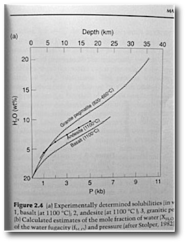
I’ve been reading a textbook on ore-forming processes as part of an attempt to get a little more fluent in geology, and I ran across a plot that is certainly well known to many, but was an eye-opener for me:

The plot charts the solubility by weight of water in several common igneous rocks as one moves deeper into the lithosphere. The take-away message is that even at modest depths, rocks can be very heavily hydrated and are capable of harboring a very large amount of water.

The plot brought to mind something that, to my highly inexpert eye, has always seemed a remarkable coincidence. The volume of water in Earth’s oceans has an average depth of ~4000 meters, leading to a sea-level that does a pretty fair job of outlining the continental margins (which mark the boundaries between denser (but thinner) basaltic crust and lighter (but thicker) granitic crust. Only about 20% of the total continental crust is overlaid by water.

In the extrasolar planet context, an interesting question is whether the situation here on Earth is unusual. Many of the planets that Kepler has found (and will be finding) contain water mass fractions that are considerably larger than Earth’s. Is it reasonable to expect that they’ll have deep oceans that uniformly cover the planets, or is there some sort of mechanism involving water of hydration that maintains a seafloor-continent dichotomy even in the presence of a lot of water? As far as I can tell, this question hasn’t been answered definitively.

The naive answer seems to be along the following lines. Imagine that a terrestrial planet forms in such a manner that the mantle rock is heavily hydrated. Given that mantle rock can easily retain a water mass fraction measured in tens of percents, one could start out with a planet that contains many oceans worth of water, but in which substantial portions of the surface are dry.

When rock melts, the water of hydration is squeezed out. (Migration of this water into the surrounding country rock leads to the mineralized veins that are the basis for many of Earth’s great ore deposits.) On an ongoing volume-weighted basis, most of the melting is taking place beneath the spreading centers that form the mid-oceanic ridges. Every year, of order 300 cubic kilometers of melt are produced, several cubic kilometers of which are erupted to form fresh ocean crust. Coupled with mantle convection, this means that the mantle unburdens its water on a timescale of order a billion years. Some of the water is subducted back down, but this sink is less effective than the source, meaning that the water likely ends up on or near the surface.

So one can imagine planets (perhaps with mantle convection less vigorous than Earth’s) in which continents are gradually submerged as water is squeezed out of the mantle. Not, perhaps, a bad way to go. The world’s best beaches are those of the Seychelles islands — a handful of granitic specks in the vastness of the Indian ocean — the highest peaks of the submerged continental Mascarene Plateau.

Press attention…

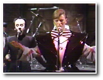
Klaus Nomi and David Bowie (Image source and backstory)

I was in the middle of my dynamics lecture this past Monday morning, explaining the Fokker-Planck approximation to the collision term on the right-hand-side of the Boltzmann equation, when my phone started buzzing and vibrating in my pocket. Good thing I had remembered to turn the volume off. Without having to look at who might be calling, I knew it was likely some media outlet, BBC? KCBS? There was a sudden, all-to-familiar sensation of queasy uneasiness which made it very hard to focus on the second-order terms I had just written on the whiteboard.

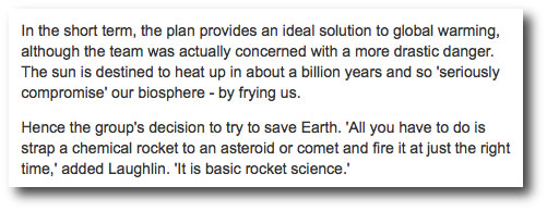
Back in 2001, I naively and foolishly spoke to a reporter at the London Observer about the “relative ease” of accomplishing strictly hypothetical orbital engineering in the context of a billion-year time frame. The resulting article (now archived by the Guardian) contained an alarmingly incorrect cognitive leap from the ultra-long term to the immediate near-term:

The misconception came exactly at the time when George W. Bush was visiting Europe, explaining his position regarding the Kyoto Protocol. The Observer story became a huge, completely nightmarish story in Europe, which then echoed across the Atlantic, where it was seized upon by the Drudge Report, Rush Limbaugh and others. Here’s an example editorial from the Manchester New Hampshire Union-Leader:

For nearly a week, the story managed to survive, zombie-like through successive news cycles. Eventually, Gary Condit appeared on the scene, and finally, the media’s full attention was diverted elsewhere.

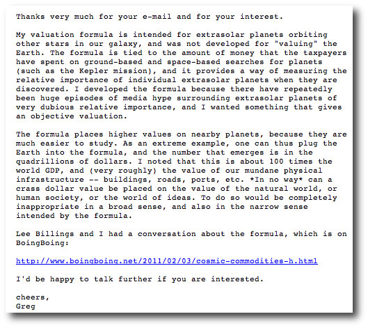
As readers likely know, I’ve been writing on this web log about a planet valuation formula, which is designed to give a quantitative assessment of whether a newly discovered planet is worthy of significant media attention. Last month, I had a detailed conversation with Lee Billings, which was published on BoingBoing as a part of Lee’s series of posts on planets (which are well worth reading!)

Several weeks after the BoingBoing article appeared, I got a very politely worded e-mail from a reporter at News of the World.

[…] I found your article on the value of the Earth which popped up on a UK blog late last week.

From what I can ascertain, your findings and formula haven’t really had the coverage they deserve in the UK media and I was hoping to rectify that…

After a look at the Wikipedia page on News of the World, my heart was pounding. “Wacko US Prof Sez: Sell Earth for 3 Quadrillion Quid!” I sat down at the computer, and it took a long time to compose a reply.

Turned out that the reporter was admirably interested in getting the story right, and the final version (which is behind a paywall) is quite fair. After all, given the possibly arch, arguably pretentious tone here on oklo.org, I did pretty much have it coming.

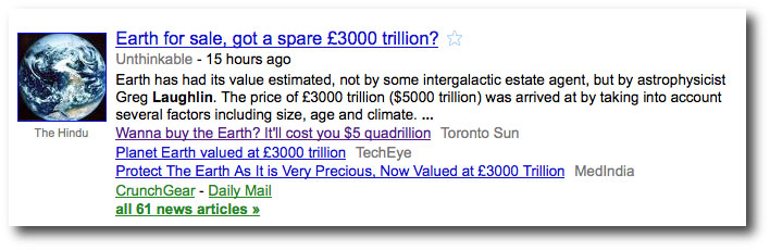
Predictably, newspapers in Britain saw the News of the World story and immediately picked it up. As is to be expected, successive iterations tend to lose focus on the exoplanets, and gain focus on the value of Earth. Radio stations are calling, trying to set up interviews about how much Earth is worth. Angry e-mails drift into my inbox. Google news is at 61 articles and counting.

I think it’s time to look into installing Google’s AdSense…

Blue straggler planets?


Image Source.

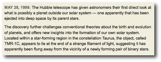
In the midst of all that excitement surrounding the Kepler data release, it was easy to overlook the article by Martin & Spruit, Inflated hot Jupiters from merger events, that showed up on astro-ph earlier this month. This paper proposes a sure-to-ruffle-feathers explanation for the radius anomalies of the hot Jupiters. The idea is that stellar mergers (arising from orbital decay in very close binaries) shed angular momentum via an “excretion” disk, from which one or more short-period giant planets manages to form. In this picture, short-period, anomalously inflated planets are large because they are young — their formation dates to the binary star merger that created their parent star, and they are headed inward for destruction on timescales significantly shorter than the typical several-billion year age of planet-bearing main-sequence stars.

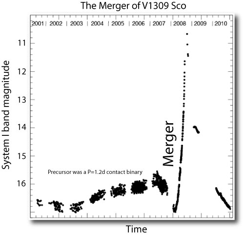
Image Source: Tylenda et al. 2010.

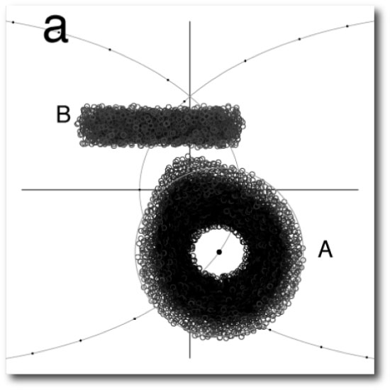
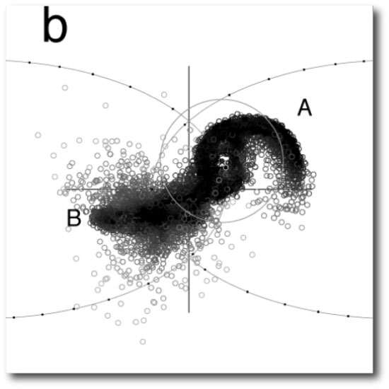
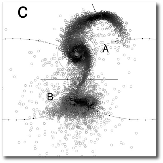
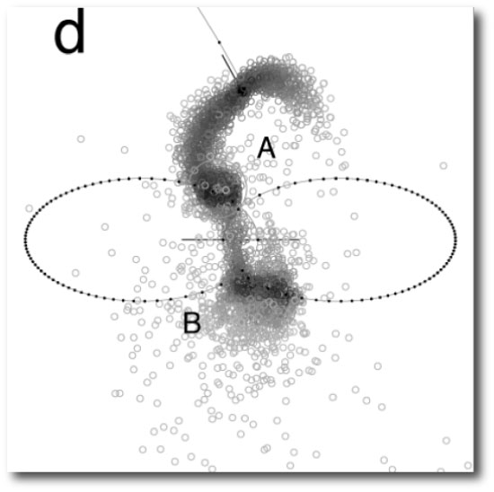
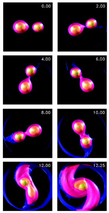
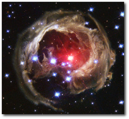
It’s believed that the anomalous novae V1309 Sco (which occurred in 2008) and V838 Mon (which made a big splash in 2002, and whose light echo is shown in the image at the top of the post) were both caused by binary mergers. In the case of V1309 Sco, the more massive of the two progenitor stars was probably similar in mass to the Sun, whereas for V838 Mon, a primary of order 8 solar masses was involved. Numerical simulations, such as the ones shown below by D’Souza et al. (2006), suggest that two distinct stars merge into a single star surrounded by a disk-like structure over an action-packed phase that lasts ~10 orbits.

The idea that merging stars can give rise to planets shows up prominently in the literature in the 1980s, with a series of papers in Soviet Astronomy by A. V. Tutukov, who had a number of speculative ideas regarding planet detection and planetary systems that have turned out to be quite on the mark — he did detailed calculations of the prospective yield of M-dwarf transit surveys, and he argued that ~25% of stars should harbor planetary systems. In several papers (including here) he advocated the idea that excretion disks can give rise to planet formation.

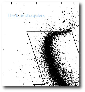
It occurred to me that in the event that stellar mergers do indeed serve as an effective formation channel for short-period planets, then blue stragglers should be very high-grade ore for photometric transit searches. The blue stragglers are main-sequence stars in globular clusters that lie above the main-sequence turn-off in the Hertzsprung-Russell diagram, and which are generally found near the cluster core. It’s believed that they owe their relative youth to being the product of binary mergers.

One of the most important early exoplanet-related results was the Gilliland et al. 2000 HST photometric survey of the rich nearby globular cluster 47 Tucanae. The Hubble telescope was trained on the cluster for 8.3 days, and time-series photometry (taken through two filters) was analyzed for ~34,000 individual stars. If the occurrence rate of hot Jupiters in 47 Tuc was similar to the occurrence rate in the solar neighborhood, then 17 transit planets were to be expected. None were found. This null result is generally attributed to the cluster’s low metallicity and to the possibility that planet formation was inhibited by the dynamical interactions and intense UV radiation that occurred during the cluster’s star formation phase.

A close up look at the 47 Tucanae color-magnitude diagram indicates that the 2-color HST imaging of cluster contains about twenty blue stragglers. Interestingly, it’s not entirely clear whether the blue stragglers have been folded for transits. In the Gilliland et al. 2000 paper, it appears that only the conventional main-sequence stars in the cluster were included in the analysis. The paper states: “For the results discussed further below only the 34,091 stars falling within a bright main-sequence box as shown were analyzed for time series.”

If hot Jupiters are commonly forming from binary merger events, then it seems like there should be a good chance that there could be a transit among the 20-odd blue stragglers observed with HST. Because this handful of stars are much smaller than the red stars at the same luminosity, the transit depths could likely be detectable, given the quality of the HST photometry and the brightness (I=16-17) of these stars. If the planet occurrence rate for merger remnants is 50% one would expect to find one transit among the tweny stars, given the ~10% a-priori geometric probability of transit. As a first step, certainly, it’ll be interesting to see whether these stars were analyzed in any of the follow-up work that was done with the Gilliland et al. dataset.

complications

Earlier this year, in the New York Times Magazine, there was a very lengthy, very glossy advertising insert devoted exclusively to high-end watches. I leafed idly through it, and picked up a new concept, that of a complication. Where watches are concerned, a complication refers to any feature that goes beyond the simple display of hours, minutes, and seconds. According to the Wikipedia,

The Patek Philippe Calibre 89 is a commemorative pocket watch created in 1989, to celebrate the company’s 150th anniversary. Declared by Patek Philippe as “the most complicated watch in the world”, it weighs 1.1 kg, exhibits 24 hands and has 1,728 components in total, including a thermometer and a star chart. Made from 18 carat (75%) gold, it has an estimated value of $6 million, and took 5 years of research and development, and 4 years to manufacture. Four watches were made; one in white gold, one in yellow gold, one in rose gold and one in platinum.

The Calibre 89’s complications include such must-haves as the equation of time (yielding the instantaneous difference between apparent solar time and mean solar time), the date of Easter, and a 2800-star celestial chart. And just imagine the convenience of being able to pull your 2.42 lb watch out of your pocket whenever the need strikes to see what century it is!

It occurred to me that the 1,235 Kepler candidates could conceivably provide a bonanza for the high-end mechanical watch industry. The candidates, with their particular periods, transit durations, transit depths, effective temperatures, and radii offer endless opportunities for unique horological complications. In this spirit, at the link below, I’ve made a 1,235-complication applet which charts the appearance and disappearance of transits, timed from the start of Kepler’s Q0. The horizontal direction is mapped to orbital period, and the vertical direction is mapped to M=R^2 in Earth units. It’s mesmerizing to watch…


Click here to watch the animation.

A planet-metallicity correlation for low-mass planets

The planet — host star metallicity connection has been one of the most secure and enduring results from the radial velocity planet surveys. In 1997, soon after the detection of the first planets, Guillermo Gonalez pointed out that the host stars were significantly enriched in elements heavier than hydrogen and helium, and suggested that a planet-metallicity connection exists.

Over the years, the correlations have been refined by many different workers, and a clear set of facts has emerged:

(1) Giant planet hosts, all the way from low-mass red dwarf stars through stars that are somewhat hotter and more massive than the Sun, tend to be metal rich.

(2) The occurrence rate for giant planets increases with stellar mass.

(3) Among stars with mass similar to the Sun, there’s no evidence that the presence of sub-Neptune/super-Earth is correlated with host star metallicity.

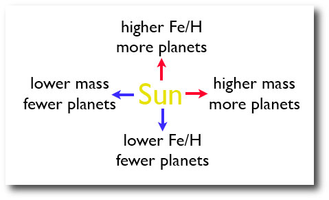
Taken together, these facts provide basic support for the core-accretion mechanism of giant planet formation. A planet like Jupiter forms by first assembling a core of icy/rocky/metallic material. When the core mass grows to of order 10-20 Earth masses, the core gains the ability to very rapidly accrete hydrogen and helium, and increases its mass by a significant, multiplicative factor to become a full-blown giant planet. Core accretion is a threshold phenomenon in the sense that the eventual presence or absence of a giant planet depends sensitively on whether the core is assembled while nebular gas is still present. Sufficiently rapid core growth is strongly aided by larger disk masses (which is the source of the planet-stellar mass connection) and by larger surface densities of solids in the disk (which is the source of the planet-stellar metallicity connection).

“Better late than never.” You hear that a lot when the chronic under-performance of super-Earths and sub-Neptunes is being discussed. The planet census makes it clear, however, that when not pressured to succeed while the gas is still there, sub-Neptunes and super-Earths regularly grow to 5-15 Earth masses and migrate to various locations in protoplanetary disks. The observations, furthermore, show that for host stars lying close to a solar mass, there’s no evidence for any metallicity dependence in the occurrence rate of these lower-mass planets.

At some point, however, metallicity has to play a role. An early-bird Population II star with [Me/H]=-3 started out with only ~0.1% as much iron, molybdenum, oxygen and carbon as did the Sun. Super-Earths won’t be found orbiting such stars because the raw planet-building materials flat-out weren’t there. Likewise, for low-mass disks orbiting low-mass stars, the overall metal budgets are tight enough that it’s quite reasonable to expect that a planet-metallicity connection for non-giant planets should be detectable.

Last year, Kevin Schlaufman and I looked into this issue and we found a tantalizing hint that among the red dwarf stars, a planet-metallicity connection does exist for planets with ~Neptune mass and below. The statistics were too sparse, however, to have anything more than ~1-sigma confidence.

Enter the Kepler results. In the course of an afternoon, 1,235 planet candidates flooded the market, completely upending the old business-as-usual model for the planet hunters. Correlations no longer emerge, they pop out.

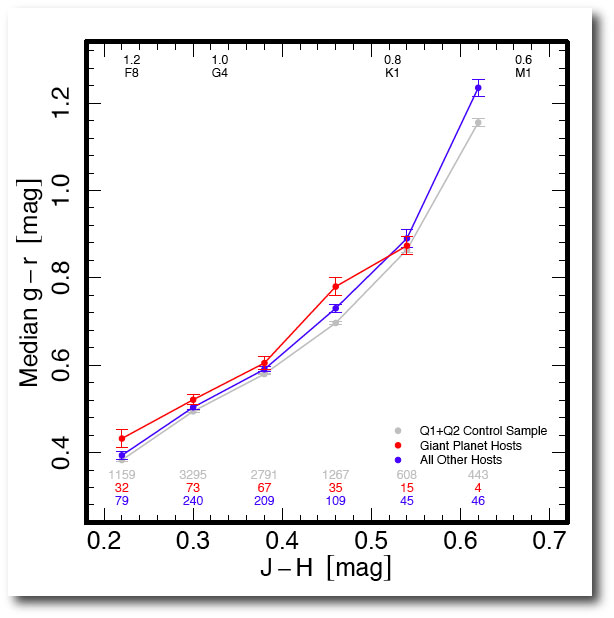
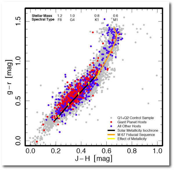
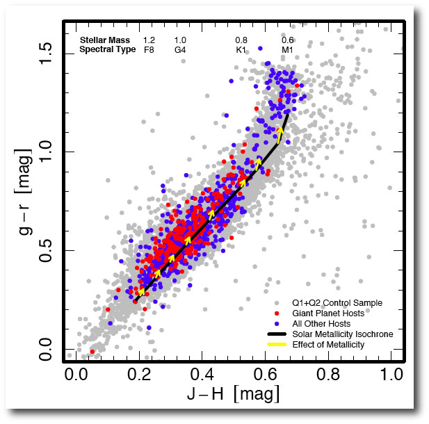
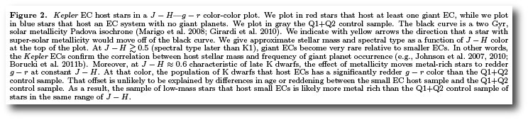
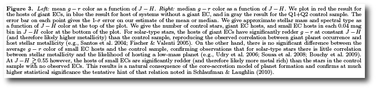
In addition to being numerous, the Kepler stars are quite well characterized, and Sloan photometry has been published for the ~150,000 stars with Q1+Q2 public-domain light curves. At a given J-H color (obtained from the 2-Mass catalog) a star’s Sloan g-r color is significantly dependent on metallicity (see, e.g. here). It’s thus informative to make JHg-r color-color plots with (1) a control sample of 10,000 stars drawn from the Kepler 156K star target list, (2) the Kepler giant planet (Rp>5R_earth) hosts, and (3) the Kepler low-mass planet (Rp<5R_earth) hosts:


These plots, which are from a paper that Kevin and I just submitted to the Astrophysical Journal, demonstrate quite convincingly that a metallicity correlation does exist for low-mass planets orbiting lower-mass stars. (The correlation starts to kick in below ~0.8 solar masses.) Assuming that the probability of forming a planet is proportional to the total amount of solids in its protoplanetary disk, the correlation indicates that a late K-dwarf with 70% of the Sun’s mass needs to have a metallicity [Fe/H]=0.15 to have the same chance of forming a planetary system as a solar metallicity star of similar mass.

I’m pretty excitied about these results. A quantitative statistical link between relative disk conditions and planet outcomes for the huge super-Earth population gives us direct information about how the really interesting systems — the ones harboring large terrestrial planets — are assembled.

We’ll put the paper on astro-ph once it’s gone through review. It contains a lot of work to establish that the correlations are real, rather than due to reddening or the various observational biases inherent in the Kepler target list.

commensurabilities


Last August, SFMOMA put on an exhibition that featured a number of Chuck Close’s hyperrealistic portraits. It was interesting to study the sudden transition between a patchwork of acrylic brush strokes, as in the cell-phone close-up snapshot just above, and an image that makes sense as a whole.

The recent public release of the Kepler data triggers an effect that’s a bit like stepping back rapidly from one of Close’s portraits. Suddenly, a huge swath of the planetary distribution connects with a larger picture. This effect holds especially true when one looks at the list of systems that harbor multiple transiting candidates.

With the census of radial velocity planets, it’s often quite difficult to determine whether a signal is originating from a single planet on an eccentric orbit, or a pair of planets participating in 2:1 resonance. The only really well-characterized unambiguously resonant RV system is Gliese 876, where the combination of large Ks, a long observational base, and rapidly unfolding 30-60-120d orbits has allowed the dynamics of the resonance to be revealed in detail.

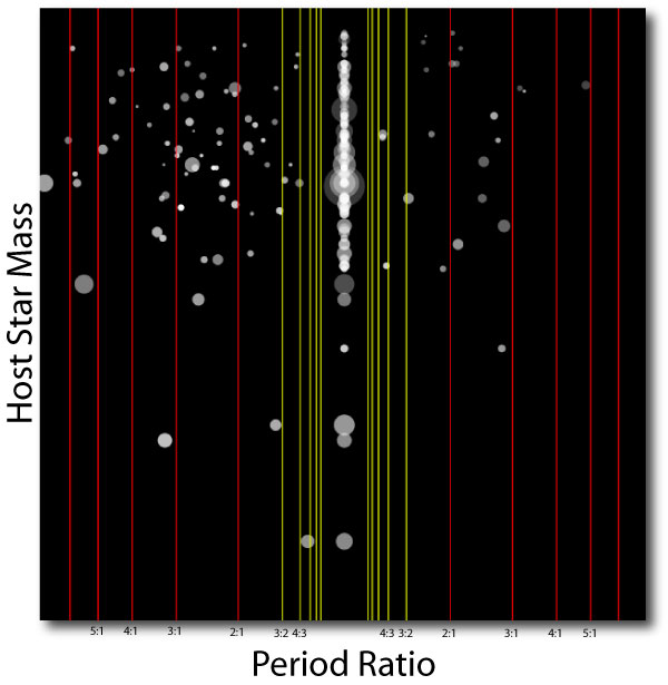
The 115 Kepler two-transit systems indicate right away that systems like Gliese 876 are intrinsically rather rare. In the illustration below, I’ve taken each of the two-transit systems, and identified the larger member of the pair. I’ve then plotted the period ratio, P_small/P_large as the x coordinate, the parent star’s mass as the y coordinate, the temperature of the planets as a grayscale (saturating to white at 1500K), and the sizes of the symbols in proportion to the observed radii.

The immediate impression from the diagram is that the systems are not overwhelmingly clustered around the simple integer commensurabilities. Low-order mean-motion resonances among the extrasolar planets are the mild exception, and not the rule.

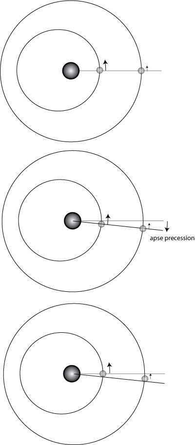
That said, the resonant systems are clearly present. Of the forty 2-transit systems with inner-outer period ratios lying between 2.0 and 3.0, six of them have period ratios between 2.02 and 2.05. The chances of a concentration like this occurring purely by chance is considerably less than 1%. Furthermore, the fact that the clustering occurs a percent or two above the exact 2:1 commensurability can be understood in terms of the dynamics of resonance. When one has two massive planets deep in a resonance, with a significant angular momentum deficit, then the system apse precesses in a retrograde direction (as is the case with Gliese 876). The resonance is controlled by a restoring force that drives conjunctions to occur at periastron. This means that if one observes along a fixed line of sight, then the inner planet is seen to orbit a bit more than two times as often as the outer planet.

An analogy?

Image Source.

If one looks at planetary systems from the “modern” point of view provided by the HARPS survey and the results from Kepler’s recent data release, our own solar system looks pretty strange. In the Sun’s case, the frequently planetiferous orbital zones inside of P=50 days are completely, mysteriously barren. The orbital region inside P<3000 days is also almost entirely bereft, with just a few iron-silicate dregs totaling less than two Earth masses. Out in the boondocks, however, the Sun’s harbors a giant planet that managed to accumulate lots of gas, yet paradoxically didn’t manage to migrate a really significant distance.

It will take more time to determine whether the solar system is really all that weird, but with each passing month’s accumulation of fresh exoplanets, our eight-planet set-up manages to seem slightly less ordinary. Jupiter, for example, induces a 12 m/s velocity half-amplitude, and the high-precision radial velocity surveys have been operating for long enough so that if true-Jupiter analogs were the rule, then we’d perhaps be hearing of more of them being detected.

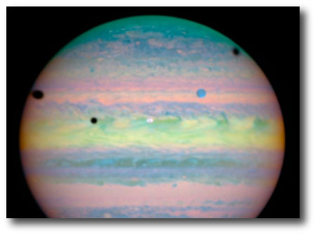
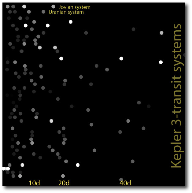
The Kepler multi-transiting candidates correspond to systems that are completely alien when compared to MVEMJSUN, but they are much more familiar when compared to the regular giant planet satellites — the moon systems of Jupiter, Saturn and Uranus. In each of these cases (and despite a factor-of-twenty difference in mass between Jupiter and Uranus) the characteristic orbital period is of order a week, and the characteristic secondary-to-primary mass ratios are of order a few parts in 100,000. For example, Ariel, Umbriel, Titania and Oberon have mass ratios of 1.6e-5, 1.4e-5, 4.0e-5, and 3.5e-5 relative to Uranus, and their orbital periods are 2.52, 4.14, 8.71, and 13.46 days. In the Jovian system, the satellite/Jupiter ratios for Io, Europa, Ganymede and Callisto are 4.7e-5, 2.5e-5, 7.9e-5, and 5.8e-5, with corresponding orbital periods of 1.76, 3.55, 7.15, and 16.68 days.

In the plot below, I’ve taken the 45 three-transit systems from Kepler’s list, and plotted the orbital periods of their constituent planet candidates along the x-axis. The colors of the points are given a linear gray-scale, with black corresponding to a planet-to-star mass ratio of zero, and white corresponding to a planet-to-star mass ratio of 1.0e-4 or larger. I’ve converted radius to mass by assuming M=R^2 when mass and radius are expressed in Earth masses and Earth radii.

It’s interesting to speculate whether the commonality between the regular satellite systems, and the teeming population of Super-Earth/Sub-Neptune class systems might be more than just a coincidence…

The Mass-Period Diagram


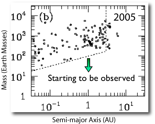
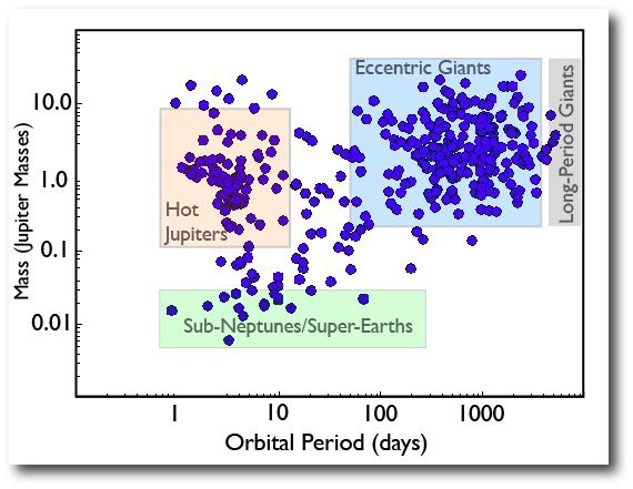
The extrasolar planets constitute a fast-moving field. I was looking at the slides from a talk that I gave in early 2005, in which I showed the then-current, now hopelessly outdated, mass-period diagram for the known extrasolar planets:

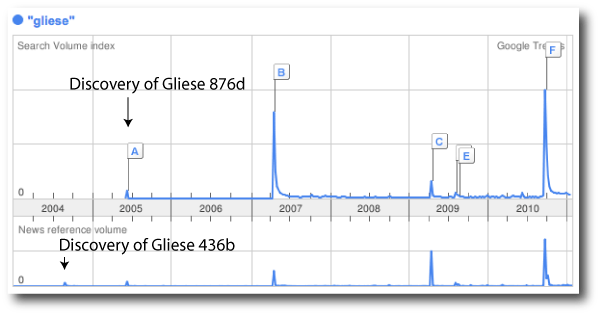
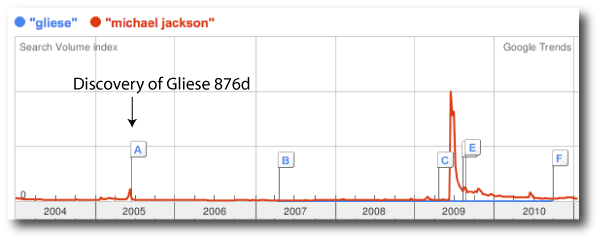
At that time, the name “Gliese” had barely edged into the public consciousness, as a Google trends and news reference diagram illustrates:

The discovery of Gliese 436b occurred in the summer of 2004, and was the first Neptune-mass extrasolar planet found. The following summer saw the announcement of the first unambiguous “super-Earth”, Gliese 876d, which generated a blip in search volume in addition to news volume. The discovery of Gliese 876d might have been a bigger story, had it not shared a news cycle with Michael Jackson:

In early 2005, there was essentially no hint of the enormous population of sub-Neptune/super-Earths lying just below the threshold of detectability. Population synthesis models for extrasolar planets were doing an excellent job of reproducing the distribution of hot Jupiters, the period “desert”, and the population of eccentric giants, but at that time, the smart-money expectation was that the pickings would be rather slim in the hot sub-Neptune regime. (It was also believed that the detection rate would pick up substantially once truly terrestrial planets became observable.)

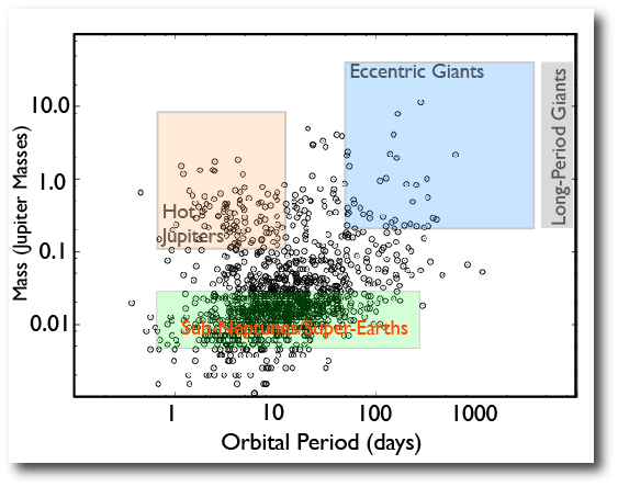
Mayor et al.’s announcement in 2008, therefore, came as a real bombshell. The Geneva Team made the startling claim that a very substantial fraction of stars in the solar neighborhood harbor at least one planet with Neptune mass or less, with an orbital period of fifty days or less. Their claim is equivalent to the statement that in a volume-limited survey, the number of planets in the green box of the diagram below is of order five times greater than the sum of the number in the peach box and the blue box.

In the diagram above, the population of planets known in 2010 is plotted. There’s a bulky cohort of RV-detected eccentric giants (Msin(i)’s), a lot of hot Jupiters from the transit surveys, and a respectable, but still sparse population in the sub-Neptune/super-Earth category. The Geneva claim was based primarily on signals that are emerging in the HARPS data, rather than solid published planets.

Fast-forward to last week. Kepler has suddenly augmented the planetary census by more than a factor of three. If we estimate masses through the simple relation Mpl=Rpl^2, then we can plot the Kepler candidates on the mass-period diagram. Detection biases etc., etc. aside, it’s abundantly clear that there is indeed a huge population of objects in the ground staked out by the Mayor et al. 2008 announcement:

Scatter Plots


In trying to make sense of the flood of new Kepler results, the very first order of business is to run through the various scatter plots to get a sense for the distributions, to look for correlations, and to test pet theories.

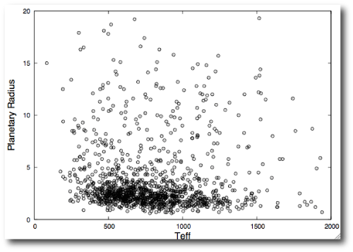
Kevin Schlaufman has made a useful formatted electronic table that joins Tables 1 and 2 from the Borucki et al. (2011) paper. Sifting through this table alone, notwithstanding the gigabytes of light curves currently available for download, there’s lots of very interesting stuff. For example, plotting planetary effective temperature vs planetary radius shows that as expected, there are a lot more small planets than large planets:

If we were looking at a complete volume-limited survey of planets, then this plot would have an interesting interpretation. The downward sweep of the main locus suggests that hot planets, by and large, tend to be smaller than cooler planets. The natural interpretation would be that we’re seeing a signature of evaporation — hence CoRoT-7b, AKA “Planet Freeport-McMoran” is small, whereas Gliese 1214b AKA “Planet Dasani” is relatively large by comparison. (Corporations interested in paying for product placements on oklo.org, please contact me directly.) Sadly, however, before jumping to conclusions, one has to worry about a whole host of possible gotcha-style observational biases. Small planets are harder to detect via transits, meaning that more orbits are required to reach given signal-to-noise, meaning that small planets are more likely to be found on short-period orbits. My gut feeling is that these effects might not be strong enough to completely wipe out the observed correlation, but it’ll take a lot of careful Monte-Carlo work to understand for sure.

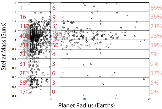
I’ve got some unhedged exposure to the planet-stellar mass correlation. The idea is that if core accretion is zeroth-order correct, then it should be easier to form giant planets in orbit around more massive stars. If this hypothesis is correct, then the giant planet fraction (defined as planets having radii greater than 5 Earth radii divided by the total number of planets) should increase as one increases the mass of the host star. Again, if one lives dangerously, throwing caution regarding biases completely to the wind, this seems to be the case with the 1235 Kepler candidates:

A Multiplexed Orrery

The planetary disturbing function describes the time-dependent perturbing potential of one planet acting on another. The disturbing function dictates the non-Keplerian evolution of planetary orbits, and while it’s conceptually simple, it’s a triumph of analysis that it can be written down as a function of the planetary orbital elements themselves.

In large part, celestial mechanics consists of choosing the right terms in the disturbing function for a particular planetary configuration, and then working out the simplified motion that arises from the chosen terms. With this program, phenomena ranging from the “Great Inequality” of Jupiter and Saturn to the possible eventual ejection of Mercury from the Solar System can be isolated and understood.

Wednesday’s Kepler data release spills a nearly overwhelming number of new multiple-planet systems into the public domain. The data include 115 candidate double-transit systems, 45 triples, 8 quads, and one each with five and six transiting planets. Precise timing measurements make all of these set-ups amenable to analysis. Correct case-by-case invocation of the disturbing function, along with an account of tidal dissipation when relevant, will generate a deep understanding of what these planets are doing, and how they got to their present state.

That’s more than a few days work. In the interim, Dan Fabrycky has created a mesmerizing video (click here for the YouTube link) which shows a wide selection of the new multi-planet systems running through their orbits for the duration of the nominal Kepler mission. It’s a multiplexed digital update of the classical clockwork orrerys that mechanically integrated the motion of those old-fashioned planets in our own solar system.

Where to start?

At 5pm PST yesterday afternoon, a series of papers from the Kepler team were released on astro-ph. These include the Borucki et al. overview of the full data set from the first four months of observation, as well as articles that delve more deeply into the results. It’s hard to know quite where to begin. In a field that’s seen more than its share of hype and hyperbole, these papers and the accompanying data represent a watershed. The most interesting facets of the galactic planetary census can now be downloaded onto your hard drive — either in the form of raw light curves or as a ready-mixed compilation of over a thousand planets. I guess it’s time to stay up late…

Earlier this year, while putting together my slides for a UC Berkeley astronomy colloquium, I got the list of asteroid discovery dates from the Minor Planet Center. Back in 1801, the discovery of Ceres was every bit as big a deal as the discovery of the first extrasolar planets, so I thought it would be interesting to compare the progression of the asteroid discoveries with that of the extrasolar planets.

The first four asteroids, 1 Ceres, 2 Pallas, 3 Juno, and 4 Vesta were all discovered within a few years of each other, and then there was a surprisingly long gap until the discovery of 5 Astraea in 1845. Here, (courtesy of the Wikipedia), are the relative sizes of the first 10 asteroids in comparison to the size of Earth’s Moon:

Starting in 1847, asteroid detections began ramping up, and by 1857, there were enough examples for Daniel Kirkwood to notice gaps in the distribution which he (correctly) suspected were due to orbital commensurabilities with Jupiter.

Source: D. Kirkwood, 1867 AAAS Proceedings

With the extrasolar planets, the shape of the discovery histogram is strikingly similar. The pace of events, however, has unfolded five times faster, with the gap between the discovery of HD 114762 b and 51 Peg b being followed by a steady ramp-up in the pace of confirmed detections. There are a lot more astronomers now than there were in the 1800s.

In my Berkeley talk, I remarked that if things were to continue at the 5x faster rate, then 2011 should see the first discovery of a pair of planets in a Trojan configuration, echoing the discovery of the first Trojan asteroid, 588 Achilles, by Max Wolf of the Heidelberg Observatory in 1906.

Amazingly, it looks as if a pair of co-orbital “Trojan” planets has been found by Kepler. As detailed in the Lissauer, Ragozzine, Fabrycky et al. arXiv1102.0543 paper, The KOI 730 system contains transiting candidates with periods of 7.38, 9.84, 9.85, and 14.78 days — fully consistent with a 3:4:4:6 resonance:

The two middle planets (red and blue) in the configuration are participating in what are likely to be wide tadpole oscillations with respect to the equilateral equilibrium, like Hector chasing Patroclus around inside the Trojan Horse.


The above figures are adapted from a paper that John Chambers and I wrote in 2002 that explores the different flavors of one-to-one resonance that might exist among the extrasolar planets. I’m eager to sift the Kepler data to search for examples of the one-to-one “eccentric resonance” in which two planets share an orbital period and toss their orbital angular momentum back and forth like a hot potato:

It is mesmerizing to bring the KOI-730 candidates up in the systemic console, and watch the stability integration (try integrating for 500 years with an output frequency of 0.01 years). If one interprets the radial velocity wave-form as a audible signal, the system is simultaneously playing a fourth and an octave, with the longer-period libration distinctly heard as an unsteady vibrato.

A 10-second .WAV file (created with the Systemic Console) is here. This should play in your browser when the link is clicked.

It’s also interesting to note that the first clear picture of an asteroid was taken in 1992 by the Galileo probe, which passed close to 951 Gaspra on its way to Jupiter.

Pushing the five-fold increase in pace to its natural conclusion, means you should be sure to check this site in 2028…

A quarter-million dollar world


Image Source.

The Kepler Candidates were just announced! My immediate sensation at seeing a copy of the associated paper is not unlike those cheesy contests where you’re allowed 60 seconds in a grocery store to grab whatever you can grab for free.

The most remarkable and unexpected development seems to be contained in Table 6 of the paper. Here, it looks as if candidates identified during the first four months of data collection have had their confidence levels increased through the use of additional transit measurements taken after September 16th, 2009. This allows for the identification of fifty candidate planets that might be considered prospects for potential “habitability”.

I ran the fifty planets in the table through my valuation formula (see here, and here.)

The total value of the planets in Kepler paper’s Table 6 is USD 295,897.65. As with most distributions of wealth, this one is highly inequitable — the most valuable planet candidate in the newly released crop is KOI 326.01, to which the formula assigns a value of USD 223,099.93. Assuming 5g/cc density, this planet has a mass of ~0.6 Earth masses, which is actually a little on the low side as far as the valuation formula is ensured. Nevertheless, USD 223,099.93 is a huge increase in value over Gl 581c, which charts at USD 158.32.

Back in 2009, I wrote that (in my opinion) the appropriate threshold for huge media excitement is USD 1M. With the planets in Table 6 of the paper, we are starting to get very close to that.

Here are the planets in the table with a formula valuation greater than one penny:

(These numbers are associated with a little bit of uncertainty. I’m using Kepler magnitudes rather than V magnitudes, and assuming 5 gm/cc. I’m also assuming that stellar mass goes as stellar radius. Running a cross correlation with the other tables in the paper will change the values slightly, but not substantially.)

Flowchart


The whole astronomical community is buzzing with anticipation over the imminent release of the unredacted First-Run Kepler results — all of the good stuff that was held back from the data release that occurred last June.

One can only imagine what might be contained — multiple-planet transiting systems, giant planet satellites, potentially habitable planets transiting low mass stars, a definitive answer to the super-Earth occurrence rate (to name but a few).

Once the candidates hit the stands, there will be a rush to skim the cream, and a mobilization of follow-up observational campaigns to capitalize on the best opportunities in the data set. With this eventuality in mind, Konstantin Batygin and I have prepared a follow-up characterization flow chart to aid fellow exoplanet prospectors in sifting potentially interesting systems — a template for the treasure map. As always, keep in mind that the brighter the individual parent star, the better the chances for the most interesting planetary characterizations.

Click here for a legible full-size version of the flowchart. (The paper containing it is focused primarily on the rather remarkable things one can do with tidally evolved multi-planet RV-detected systems. It’s been accepted to the Astrophysical Journal, and will appear on astro-ph shortly. It’s available now for download from oklo.org.)

It’s Ohmic


NOAA Weather prediction is performed continuously by two IBM Power 575 Supercomputers named Stratus and Cirrus, each carrying out 69.7 trillion calculations per second. These machines each run 20 concurrent models for a global ensemble forecast. Approved production models run on Stratus, and development codes run on Cirrus. Huge volumes of this-just-in updates to the world’s atmospheric conditions pour in constantly from satellites, radiosondes, aircraft, ships and ground stations. The resulting predictions tend to be pretty good to about five days out:

Weather prediction would get a lot harder if the atmosphere was partially ionized. Not only would the ground stations melt, but the wind would no longer be able to blow freely through Earth’s magnetic field lines, which in turn would start to behave like rubber bands that resist being stretched and squeezed. The charged wind, furthermore, would experience Ohmic resistance that would create local heating.

On hot Jupiters, temperatures are high enough so that atmospheric alkali metals such as sodium and potassium are starting to ionize. This effectively guarantees that it’s necessary to do radiation magnetohydrodynamics in order to understand how these planets really work.

In a paper published last year, Konstantin Batygin and Dave Stevension showed that Ohmic dissipation is a very attractive mechanism for providing an extra energy source that inflates hot Jupiters and contributes to the bizarre range of radii exhibited by the transiting planets (radii that have caused a lot of consternation among those who tend to worry about such things).

Konstantin’s paper got me thinking about ways to test the Ohmic dissipation hypothesis. I wrote up some initial thoughts in this post from last summer. I’ve since worked things out further in collaboration with UCSC Physics Undergrad Matteo Crismani and with Fred Adams. We have a new paper on the topic that’ll be up on astro-ph later today.

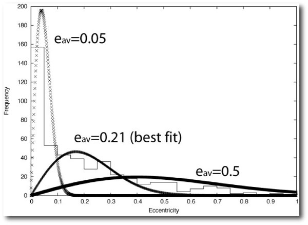
We started with the data in the plot shown above, namely the disparate collection of transiting planets with well-measured masses and radii. We computed the radius anomaly for each of these planets, that is, the difference between a plain-vanilla structural model for a solar-composition planet with the observed mass and insolation and the actual observed radii.

These radius anomalies show a strong correlation with the amount of energy that they receive from their parent stars. If one examines power-law fits, it turns out that radius anomalies scale with temperature to the 1.4+/-0.6 power.

Our bottom line is that this power-law dependence is very much in line with what one might expect from Ohmic heating (if the back reaction of the magnetic field onto the wind speed is taken into account), and my guess is that Batygin and Stevenson have taken out a large chunk of the radius problem. (See also, their very recent follow-up paper with Peter Bodenheimer).

Our paper contains several pages of details that might not be appropriate for a family-oriented site such as oklo.org, so if you’re interested, then by all means download the .pdf and have a look…

NLG

Here’s a selection of lead-off introductory lines from discovery papers of a completely random sample of planets announced in 2010:

With the discovery of extrasolar planets during the past 15 years, it has now become evident that our solar system is not unique. Similar to our Sun, many stars are believed to be hosts to giant and/or terrestrial-class planets and smaller objects.

In recent years, extending the threshold for exoplanet detection to yet lower and lower masses has been a significant endeavor for exoplanetary science. As at 2010 October, 31 exoplanets have been published with minimum (i.e., m sin(i)) masses of less than 20 Earth masses.

Radial velocity (RV) searches for extrasolar planets are discovering less massive planets by taking advantage of improved instrumental precision, higher observational cadence, and diagnostics to identify spurious signals. These discoveries include planets with minimum masses (M sin i) as low as 1.9 Earth masses (Mayor et al. 2009) and systems of multiple low-mass planets (Lovis et al. 2006; Fischer et al. 2008; Vogt et al. 2010). To date, 15 planets with M sin(i) < 10 Earth masses and 18 planets with M sin(i)=10–30 Earth masses have been discovered by the RV technique (Wright et al. 2010, Exoplanet Orbit Database10).

Ground-based transit surveys have been very successful at discovering short-period (P < 5 days) transiting extrasolar planets (TEPs) since 2006.

There has been a rapid increase in the number of transiting planets discovered each year due to dedicated ground– and space– based surveys: HAT (Bakos et al. 2002), TrES (Alonso et al. 2004), XO (McCullough et al. 2005),WASP (Pollacco et al. 2006), CoRoT (Baglin et al. 2006) and Kepler (Borucki et al. 2010). This trend looks set to continue, with the discovery of over 35 new planets published already this year (mid 2010), which represents more than a third of the total number of transiting planets known.

These soothing, robotic cadences are familiar to everyone who writes introductions and discussions for planet discovery papers. Those astronomers write prose with machine-like precision. Machine-like. Hmm…

Last year, after one of our “Wouldn’t it be cool if?” conversations, Stefano Meschiari and I decided to take up the daunting challenge of developing an NLG software package that can analyze radial velocity data, “discover” any statistically significant planets contained therein, and then write a publication-quality paper, that includes a human-readable introduction and analysis.

Stefano did the development work to produce an remarkable first-draft package, which is named “BAM” — short for Big Automatic Machine. Check out this screen-capture video of the systemic console hooked up to the BAM:
The Big Automatic Machine in action

There are certain advantages to having a computer write planet detection papers… BAM can go out on the Internet and scour the catalogs and the literature, which allows it to place new planets smoothly into the broader context. By looking at where new planets fall within the confines of all the known distributions, it can spot trends, peculiarities, and facets of interest.

As an example, for the planets discussed in Stefano’s latest lead-authored paper, BAM notices that several of them fall in a somewhat sparsely populated region of the mass-period diagram:

With a little coaxing and advice from its human minders, it now produces the following discussion:

All the planets presented in this paper lie well within the existing exoplanet parameter envelopes (Fig. 15). Several of them lie in the so-called “desert” in the mass and semi-major axis distribution of extrasolar planets (Ida & Lin 2004). Monte-Carlo population synthesis models for extrasolar giant planet formation tend to suggest that planets migrate relatively rapidly through the period range between 10 and 100 days, and, in addition, often grow quickly through the mass range centered on the Saturnian mass. In the context of the overall planetary census, these four new planets help to further elucidate the various statistical properties of exoplanets. In particular, the discovery of multiple-planet systems helps in further characterizing the number of stars hosting multiple planetary companions and any correlations emerging in the distribution of orbital elements as suggested by observational clues (e.g. Wright et al. 2009).

With extrasolar planets as the topic, art retains a certain precedence over craft, and for the foreseeable future, BAM will be stuck with a learner’s permit — only allowed to drive if there’s a licensed driver in the car. I can imagine more mercenary, lawyerly, applications, however, where it will be able to really come into its own.

BAM, with its perfect command of LaTeX, its dry analytic mindset, and its cautiously factual discussions, writes prose that is pretty much the opposite of the writing that you’ll find in Jack Keroac’s On the Road. From the Wikipedia:


Keroac completed the first version of the novel during a three-week extended session of spontaneous confessional prose. Kerouac wrote the final draft in 20 days, with Joan, his wife, supplying him bowls of pea soup and mugs of coffee to keep him going. Before beginning, Kerouac cut sheets of tracing paper into long strips, wide enough for a type-writer, and taped them together into a 120-foot (37 m) long roll he then fed into the machine. This allowed him to type continuously without the interruption of reloading pages.
In the mid-1950’s, at the urging of Allen Ginsberg and William Burroughs, Keroac compiled a list of “essentials” for writing the spontaneous prose that comprises On the Road and his other work. Taken as a set of instructions, they seem almost perfectly designed to defy machine implementation in an NLG program. Take for example, the prescription for implementing proper structure:

STRUCTURE OF WORK
Modern bizarre structures (science fiction, etc.) arise from language being dead, “different” themes give illusion of “new” life. Follow roughly outlines in out fanning movement over subject, as river rock, so mind flowover jewel-center need (run your mind over it, once) arriving at pivot, where what was dim-formed “beginning” becomes sharp-necessitating “ending”and language shortens in race to wire of time-race of work, following laws of Deep Form, to conclusion, last words, last trickle-Night is The End.
One gets the feeling that the computers are still a decade or so away…