oklo – Page 27 – delineating connections

time series

May 1, 2007

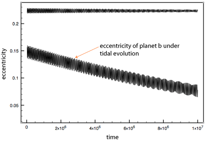
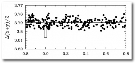
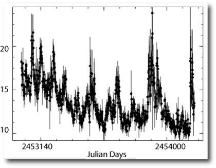
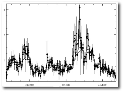
It’s remarkable how Keplerian fitting functions can be pushed to model a wide variety of time series. Anyone recognize this particular data stream?

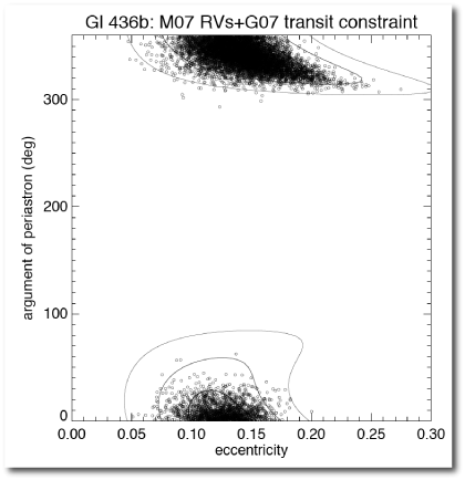
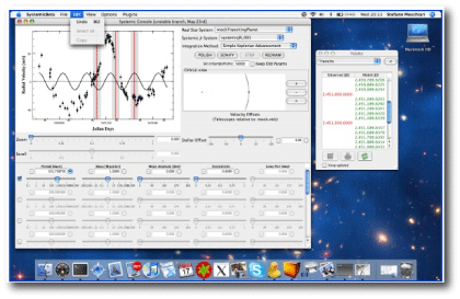
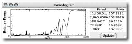
It shows complicated behavior on timescales ranging from days to years, superimposed on an autoregressive tendency. The downloadable systemic console‘s periodogram points to significant power at low frequencies, reflecting the gradual overall decline during the duration of the time series. There are also a number of distinct peaks at higher frequencies.

A crazy (read eccentric) six-planet Keplerian system does a credible job of fitting the data.

largely because the periastron passages of eccentric planets are capable of producing peaks that ramp up and then decay. To fit a particular peak, the five keplerian parameters can be varied to produce an enormous variety of waveforms.

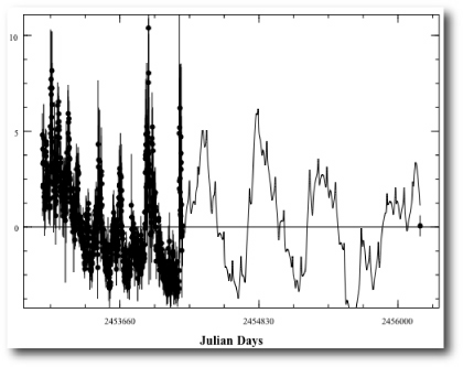
The Keplerian model can be evaluated at any forward time to make a prediction, albeit in this case, one with presumably zero physical justification…

Gl 581 — The Movie

April 26, 2007

While talking to a reporter this morning, I ventured 1000:1 odds against Gl 581 “c” harboring a clement surface or a temperate ocean-atmospheric interface. Too bad we haven’t yet tapped into the galactic market — I’d like to hedge my bet with the purchase of an appropriate derivative security.

Habitable or not, Gl 581 c is pointing toward better worlds to come. As I remarked in the past two posts (1,2), we’re guessing that “c” formed beyond the snowline and migrated inward to its current position just outside the nebulous inner boundary of the habitable zone.

Here’s a 1.1 MB animation of Jonathan Langton’s simulation of the flow pattern on Gl 581 c. The clip shows 30 hours worth of weather on our model of the planet:

First a few technical details. We model the planet’s lower radiative stratosphere with a 2D compressible hydrodynamics code. We use a time-dependent model for radiative heating and cooling. The planet is assumed to be spin-synchronous, so that it rotates on its axis once every 12.9 days. The planetary mass is five-Earth masses (I’m holding out for a transit on May 7th!), and we take a radius of 1.7 Earth radii. The orbit is assumed circular, the luminosity of the star is 0.013 solar luminosities, and the planetary “Bond” albedo is assumed to be 55%. At the layer we’re modeling, we assume a molecular weight of 25, and an atmospheric column depth of 2500 kg/m^2. This corresponds to an atmospheric pressure at the troposphere-stratosphere interface of order 400 milli bar. We assume an equilibrium night-side temperature of 250K (as a result of heat welling up from beneath).

The animation shows the sub-stellar hemisphere. The weather on the planet rapidly reaches an equilbrium flow pattern with small windspeeds (of order 3-4 m/s). The temperature at the substellar point equilibrates at 330K.

In the deeper, convective layers of the atmosphere, we expect fierce thunderstorms to occur. In analogy with thunderstorms on Earth driving anvils into the stratosphere, we model the effect of the thunderstorms by supplying a random heating term to the stratospheric flow. We definitely welcome constructive criticism of this approach, since we’re neophytes in the exo-terrestrial planet climate business. For the technically inclined, here’s a .pdf write-up that details our radiation-hydrodynamical scheme (the example planet in the write-up is HD 80606b, rather than Gl 581c, but the numerical method is the same).

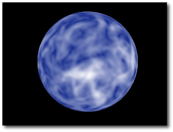
So what’s being plotted? We identified regions of higher wind speed with the formation of high water clouds (white) and regions of low wind speed with more transparent layers in which the spectrum of reflected starlight is controlled by Raleigh scattering (blue). The patterns in the atmospheric animation are thus controlled by atmospheric pressure waves and the random thermal variations driven by the thunderstorms, and not by actual advection of air.

It’s interesting to compare this with the animation of the (rotating) Earth taken by the Galileo probe as it flew by to pick up a gravity assist.

The Gliese 581 system

April 26, 2007

I’m still really jazzed that the systemic users detected Gl 581 c prior to its discovery announcement.

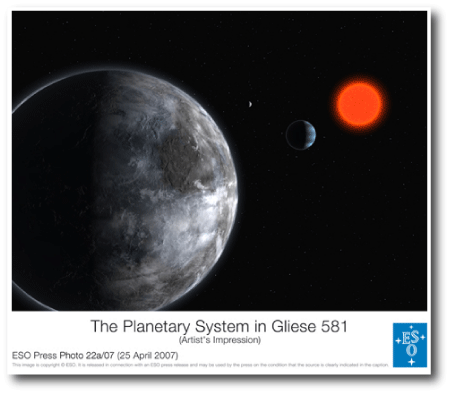
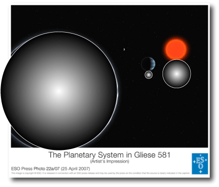
A dramatic ESO press release “Artist’s impression” of the Gl 581 system is all over the web today. It shows a planet that appears quite dry, clearly drawing on a model of in-situ formation from silicates and iron. In all likelihood, however, the planet migrated from beyond the snowline in Gl 581’s protostellar disk. It likely contains at least an Earth’s mass worth of water, and the view from space would show the upper layers of a deep and stormy atmosphere. Jonathan Langton is running hydrodynamical simulations to try to get a sense of what the weather is like on this world, and we’re hoping to have an animation up very shortly. (See this brief description of yesterday’s splash image).

Image Source.

One of my pet peeves is that it’s possible to produce far more accurate and photo-realistic press release images of extrasolar planets than is usually done. Artist’s impressions generally veer toward being luxuriously long on depicting what we don’t know and rudely short when it comes to presenting what we do know.

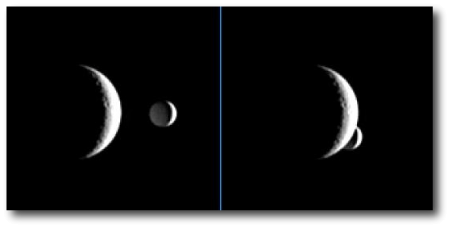
At the JPL Cassini/Huygens website, there is a trove of photos taken by the orbiter showing Saturn and its moons from different vantages and illumination conditions. The photos below were taken from a location near the ring plane, and show Rhea and Enceladus. The two pictures were taken one minute apart as Enceladus (314 miles in diameter) is occulted by the larger Rhea (949 miles across) as seen from the spacecraft.

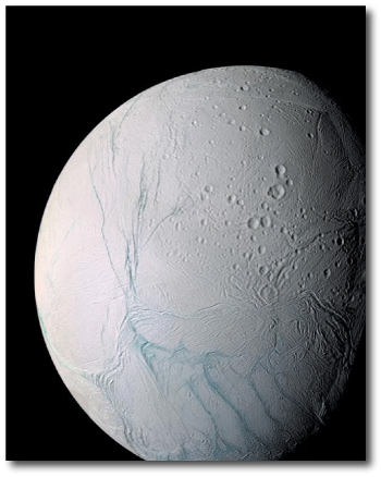
This sequence of photos makes the most of the kinds of information that we do know about extrasolar planets, namely the system geometry, the relative sizes, the orbital dynamics, and the illumination. Note how the night side of Enceladus is eerily lit by the unseen Saturn. These particular photos, furthermore, are effortlessly discrete with respect to what we don’t know about extrasolar planets, namely the geological details of the surfaces. In the absence of concrete information, the surface is perhaps better left either to the mind’s eye or to the moment when we get the real image. In Cassini’s glorious up-close view, Enceladus was revealed to be far more bizarre and interesting than anyone had imagined:

The lighting in the Gl 581 press release image is pretty weird. We’re looking straight at the parent star, and yet planet “c” is seen in quarter phase, illuminated by a source of white light placed to the right of the scene. The star, however, is thought to be single.

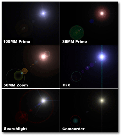
The dynamic range of illumination in the scene is way off as well. If we’re looking straight at a star, then the field of view is completely flooded, saturated with light, and replete with lens flares. Planets are always lost in the glare if you’re looking straight at a star. Since any view of a star is seen through an optical system, I think it should be possible to achieve a better sense of optical dynamical range by correctly applying lens flares. Over the next year, we’ll be looking into this in much more depth.

Image Source.

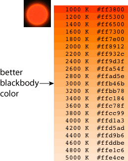
This website has an interesting discussion of how to correctly render the colors of stars. Dynamic range aside, and assuming that the star is a 3000K blackbody radiator (which isn’t quite right, but is a reasonably good approximation) the color should be a lighter shade of orange. As drawn, the color is more appropriate to the night-side glow of a hot Jupiter.

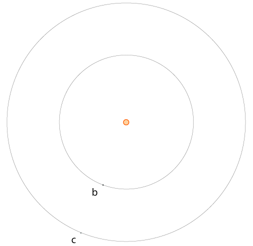
What about the perspective in the scene? At first glance, it looks like Gl 581 “b” might have been drawn a little too large. Using the information in table 1 of the Udry et al. preprint, and adopting a 1.7 Earth-diameter size for “c”, a Neptune-size for “b”, and 0.3 solar diameters for Gl 581 itself, we can draw the orbits and sizes of the planets to scale and almost have it fit correctly in an image that fits on the blog. (You may want to make your browser window wider):

In reality, because of pixelation, the tiny dots showing the planets are a bit larger than they should be. Ellipses are circles seen from an angle, so by applying a 1-dimensional re-scale with Adobe Illustrator, we can view the system to scale from a long distance away:

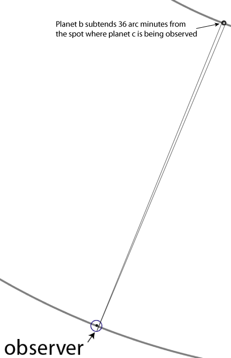
When I’m looking at the ESO press release image on my computer screen, the planet measures 7.5 cm across, and is located 45 cm from my eye. It subtends an angle of 9.5 degrees at the vantage from which its being viewed. The point of view is thus located 11 planetary radii above the surface of the planet, and drawn to scale, the geometry in the image looks like this:

As viewed from the skies of planet “c”, planet “b” subtends an angle of 36 arc minutes, and remarkably, would appear just slightly larger than the Moon appears from Earth. The parent star, on the other hand would subtend 2.3 degrees of the sky, which is about ~4.6 times larger than the Sun appears in our sky. (Given that Gl 581 “c” is in a habitable orbit, and given that the star is a red dwarf, it’s absolutely necessary to have the star fill more of the sky.) With this information, we can draw the correct angular sizes of the star and the planet “b” as seen from the vantage of the drawing. The planet “b” should be somewhat smaller than drawn, and the star should be somewhat larger. On the balance, however, the angular sizes aren’t that far away from being correct.

Gliese 581 c (confirmed!)

April 24, 2007

Gl 581 c

Big news today from the Geneva extrasolar planet search team. Using the HARPS instrument at La Silla, they have announced the detection of an Msin(i)=5 Earth Mass planet orbiting the nearby red dwarf Gliese 581. The planet has an orbital period of 12.9 days, which places it squarely within the habitable zone of the parent star.

The planet probably migrated inward to its current location from beyond the “snowline” in GL 581’s protostellar disk, and so its composition likely includes a deep ocean, probably containing more than an Earth’s mass worth of water. Atmospheric water vapor is an excellent greenhouse gas, so the conditions at the planet’s atmosphere-ocean boundary are probably pretty steamy. It’s also possible, however, that the planet formed more or less in-situ. If this is the case, it would be made from iron and silicates and would be fairly dry. It’s unlikely, but not outside the realm of possibility, that this could be a genuinely habitable world. There’s no other exoplanet for which one can make this claim. In short, it’s a landmark detection.

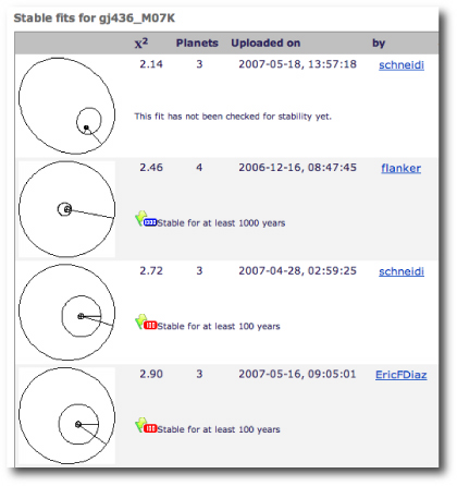
In 2005, the Geneva team announced the detection of a Neptune-mass planet in a 5.366-day orbit around the star, and they published 20 high-precision radial velocities in support of their detection. These radial velocities have been in the systemic backend database since last summer, and so naturally, when today’s detection was announced, I was eager to see the models that our users have submitted for the Gl 581 planetary system.

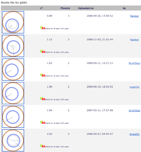
The six submitted fits with the lowest chi-square for the system — by flanker (fits 1,2), EricFDiaz (fits 3,5), eugenio (fit 4), and bruce01 (fit 6) — all contain both the known 5.366 day planet as well as a planet with properties (Msin(i)~5 Mearth, P~12.2 days) that are a near-match to the newly announced planet. In the following screenshot, I’ve highlighted Gl 581 b in blue and the newly confirmed Gl 581 c in light orange.

Eureka!

Congratulations, Gentlemen. You made the first public-record characterizations of the first potentially habitable planet detected from Earth.

I’ve gone on record a number of times to emphasize that I have no interest whatsoever in priority disputes regarding who discovered what. It’s a forgone conclusion that the Swiss should receive all of the credit for their detection. The F-test false alarm probability for the Gl 581 c signal based on the 20 originally published velocities is ~25%, and there are thousands of planets that have been submitted to the systemic backend that don’t actually exist. Nevertheless, the systemic users can take a genuine pride in knowing that they were among the first on Earth to sense the existence of this extraordinary new world. I can’t resist dusting off Sir John Herschel’s ringing exhortation to the British Association of the Advancement of Science on Sept. 15, 1846, two weeks prior to the discovery of Neptune.

The Perfect Storm

April 20, 2007

null

Most of the hot Jupiters with periods that last less than a week have orbits that are nearly circular. Tidal dissipation in a body on a short-period eccentric orbit is very strong. The net result of tidal dissipation is that energy of orbital motion is turned into heat. Io is the poster-world example of this phenomenon in our solar system.

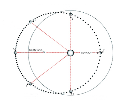
There are, however, two hot Jupiters — HD 118203b and HD 185269b — that have orbital periods of less than a week, and eccentricities, e~0.3. Indeed, a quick glance at the radial velocities for HD 185269 phased at 6.838 days shows that the variation is not a perfect sinusoid.

With its eccentricity of 0.3, HD 185269b should have long since been delivered into a state of spin pseudosynchronization, in which it spins roughly three times on its axis for every two trips around the parent star. This state of affairs prevents a steady state flow pattern from developing, and hence the weather on this world is likely to be much more interesting than on your standard-issue tidally circularized hot Jupiter. Furthermore, the amount of energy absorbed by the planet is 345% greater at periastron than at apastron, which will also contribute to a strong “seasonal” variation during the planet’s 6.838-day year.

HD 185269b was discovered by John Johnson, who has been carrying out a radial velocity survey of luminous Hertzsprung-gap stars (discovery paper here). The stars in his survey are more massive than the Sun, and are in the midst of ending the core hydrogen-burning phase of their life cycles. They’re in the process of turning into red giants, and are thus cool enough to be profitably observed with the Doppler radial velocity technique. (See this post for more on John’s survey and its implications). HD 189269 is about four times more luminous than the Sun, and so the surface of the planet should average out at ~1300 K, which is quite hot, even for a hot Jupiter.

UCSC graduate student Jonathan Langton has been making great progress in his hydrodynamical calculations of the global surface flows on extrasolar planets. His code (which he’s written from scratch during the past year) now has a more sophisticated scheme for time-dependant radiative transfer, and is ideal for simulating the weather on planets like HD 185269b, and HD 80606b that are subject to strongly varying fluxes of radiation. We’re getting close to submitting a paper on his research, which will have predicted light curves for all of the known planets that are potentially bright enough to be observed with the Spitzer Space Telescope.

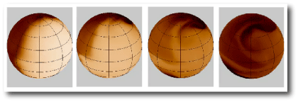
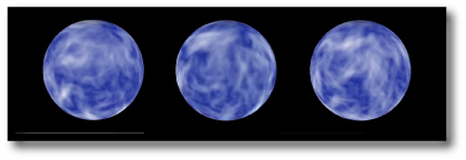
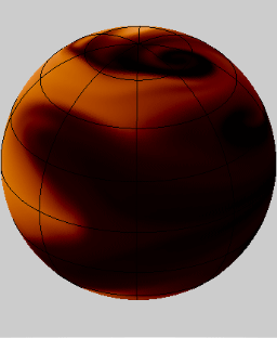
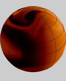
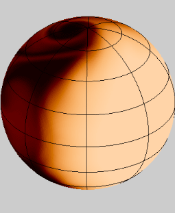
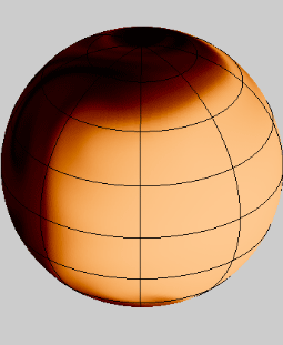
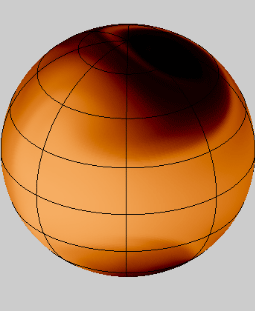
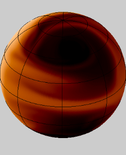
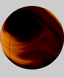
Here’s a sequence of images (each spaced by a bit more than a day) which show the global weather map for HD 185269 b as computed by Jonathan’s code. The view is from a camera that hovers above a fixed spot on the surface, and thus rotates with the planet. The color-scale is chosen to roughly approximate what the eye might see in the absence of clouds in the atmosphere. The brightest yellow regions have a temperature of ~1500K, and the coolest regions are down at ~900K. In this approximation, it’s best to think of the planet as a gigantic transparent molten marble.

In the third frame, we’re getting a good view of the heating that occurs on the hemisphere of the planet that is subject to the brunt of the insolation delivered during the periastron passage. The rapid heating of the atmosphere drives an intense global storm that is still shedding vortices and dissipating when the next wave of heating begins to hit.

It’s quite a fascinating flow, and it’s best visualized if you take the time to download the animations. Here are links to the movies: The first movie animates the temperature of the flow pattern for a full 6.838-day orbital period as viewed from a camera placed above the eastern hemisphere, and the second movie animates the temperature of the flow pattern for the same period from a camera placed above the western (opposite) hemisphere. These are 1.2 MB .avi format files. Run them on loop for a groovy lava lamp effect, and better yet, place them near a copy of the downloadable systemic console to make your desktop look like self-contained Institute for Exoplanetary Studies.

If the above .avi files don’t play on your machine, you’ll likely need to download the Xvid component for QuickTime (or an appropriate player for your OS). They are available here, and are trivial to install on Mac OSX 10.4 (Thanks for pointing me to the link, Andy!) If you can’t get the animations to play, here are links to the original .avi files for the first movie and the second movie. These are 41 MB .avi format files. I’ve put them on the UCO/Lick Server in order to keep our friends at Bluehost from wigging out and going into overload mode…

In the zone

April 16, 2007

No word yet on whether anyone flew down to Tahiti last Monday to observe GJ 674.

For Northern Hemisphere observers who want some action closer to home, there’s a cool opportunity to check HD 80606b for transits starting essentially right now.

HD 80606b is a favorite here at oklo.org (see e.g. here). The planet went through periastron passage last week, and is now just on the verge of inferior conjunction with the Earth. The a-priori geometric odds of observing a transit are 1.6%. In 2005, transitsearch.org ran a campaign on the star, and while some useful photometry was obtained, the entire transit window was not covered. If HD 80606b happens to show central transits, then the duration of the event will be ~18 hours and the photometric depth will be ~1.4%. At any one location on Earth, one would be able to observe only the ingress or the egress.

The best fit to the published radial velocity data indicates a mid-transit time of 11:07 April 17, 2007 UT. This midpoint is uncertain by roughly half a day, which means that observations starting now and ending on April 18th will be useful.

Walker Lake

April 11, 2007

Image Source

It’s hard to get a more profound sense of physical remoteness and isolation in the United States than to drive east from Walker Lake, Nevada as the Sun sinks below the western horizon. It’s like Mars.

On a transcontinental flight last month, I had a window seat away from the wing. The sky was clear over Nevada, and the sun angle was low. It was an ideal situation for high-resolution imaging of a habitable terrestrial planet. The airplane view provides an interesting link between the experience of driving across the landscape and examining the satellite photos. The area just east of Walker Lake imparts an impression of a planet that’s very different from the global idea of the “pale blue dot.” The lake itself is salty, alkaline.

The satellite and aerial photographs show that Walker Lake seems to be an evaporating remnant of what was once a much larger body of water.

Four billion years ago, Gusev crater on Mars probably looked very similar, with a sour central lake receeding with bathtub-ring clockwork.

On Mars, there are only a few spots where a high-level of zoom will reveal artificial features:

Image Source

On Earth, in the region to the East of Walker Lake, there’s very little that can’t be ascribed to natural processes. This smooth black curve seems to be a wave cut bench of the vanished shoreline:

This feature, however, would be more challenging for a planetary geologist to explain. It’s obviously younger than the channels that it cuts across. Perhaps it’s fresh material that welled up from a crack in the Earth’s crust? There are volcanos dotted across the Basin and Range province.

Just south of the region shown in the splash image for this post, there are some extremely strange landforms…

And as is often the case in planetary exploration, when one wants to see even more detail,

Bali Hai

April 9, 2007

No word yet on whether that newly discovered 11 Earth-mass (and possibly rocky) planet orbiting GJ 674 is transiting or not.

The next opportunity is coming up on April 11th 13:17 UT. Given GJ 674’s location in the sky at RA 17:29, Dec -46 54, the South Pacific has by far the best view of the next event. Anyone willing to jump on the next plane to Tahiti with a Meade LX200 and an SBIG ST-7 in their checked baggage?

The current Tahitian weather forecast for the transit window calls for scattered clouds with a 20% chance of rain:

Not exactly the best conditions for obtaining 0.5% photometry, but not completely hopeless, either. I’m interpreting the current forecast as indicating there’s a 1/3rd chance that the weather will be cooperative. This means that if you fly to French Polynesia and set up your telescope in the hotel parking lot, you’ve got a 1 in 60 shot at walking away with the biggest exoplanet discovery of the year.

Even at 60:1 odds, there’s a case to be made that the trip is a good investment. According to the CoRoT website, the CoRoT satellite will detect “a few tens” of large rocky planets for a price tag of roughly 100 Million USD. That’s ~3 million per large rocky transiting planet.

A trip to Tahiti tomorrow, on the other hand, costs out at under 4K, and involves a more clement destination than Baikonur. In fact, when I dialed up a spur-of-the-moment expedition on expedia, I was informed that the price had just gone down:

The expectation value for the Tahiti mission, therefore, is a comparative bargain at $240,000 per transiting planet.

Assuming that you can show up at LAX by ~10pm this evening (Monday) a direct flight on Air Tahiti Nui gets you in to Papeete at 5:10 Tuesday morning. There’s plenty of time to grab a taxi to the luxe Le Meridien Tahiti, where you can take a refreshing nap in your “over water bungalow” set on one of Tahiti’s few sand beaches. Follow your late afternoon dip in the pool with dinner at Restaurant Le Carre, with its trendy atmosphere and refined A la carte dishes. After dinner, there’s still plenty of time for drinks at the L’Astrolabe Bar, where they’ll likely pick up your tab while you regale the hip-yet-distinguished clientele with astronomical bon mots. Indeed, you’ll likely have an admiring circle of new-found friends as you set up your scope in the parking lot and expertly obtain darks, flats, and baseline photometry, prior to observing well into astronomical twilight.

It’ll then be time to retire to your bungalow for some well-deserved rest. You’ll have the rest of the week to analyze your data and hopefully send that discovery e-mail to the IAU. It’ll be impossible for anyone on Earth to scoop your discovery until the next transit window on April 16th, at which point you’ll be flying home (having upgraded to first class for the long-haul flight back to LA).

What’s that you say? No money for your trip? No Problem. As soon as the market opens this morning, just write a few at-the-money April calls on a precariously high-flying tech stock to raise the necessary cash.

GJ 6-7-4

April 6, 2007

Word up! Chalk a jet-fresh Neptune on the boards — the Swiss’ve done it again.

The red dwarf GJ 674 lies 14.67 light years away. Minus 49 Dec. Only 53 known stars are closer to the Sun, and at V=9.382, GJ 674 is slightly more than twice as bright in the optical as its far more famous cousin GJ 876. With ~35% of the Sun’s mass, it’s packing more heat as well.

According to the Bonfils et al. discovery preprint posted to astro-ph yesterday, GJ 674 is accompanied by a sub-Neptune mass planet on a 4.6938 day orbit. Bucking the recent trends, the paper doesn’t contain a tabulation of the radial velocities. Eugenio, however, made dextrous use of the Dexter to scrape them off the figures, and they’re now safely packaged into the downloadable Systemic Console. The star has also been added to the “Real Stars” catalog on the Systemic Backend. The internal errors on the velocities are mostly below 1 m/s, which is impressive, given that each data point is based on a 15-minute integration of a rather dim star.

This discovery is a exciting for several reasons. Most immediate, is the fact that the planet does not yet seem to have been fully followed up photometrically to check for transits. At first glance, such an effort might appear to be hampered by the fact that the star is young enough to show significant photometric variability in synch with its 35-day rotation period. A central transit, however, would have a duration of only ~80 minutes — much shorter than starspot-induced variations — and would generate a clearly detectable dip of at least ~0.5% photometric depth.

Transitsearch.org has observers in Australia, South Africa, and South America, and so I’m hoping that they can quickly take advantage of this opportunity. The next transit window is centered about 15 hours from now, on April 06, 2007 at 20:38 UT. Here’s looking at you, Perth. The ephemeris table showing all the upcoming opportunities is at transitsearch.org. Based on a radius estimate for the star of 0.35 solar radii, the geometric transit probability is ~5.0%. Roll that twenty-sided die.

It’s fair to say that the next major discovery in the exoplanet game will likely be the detection of transits of a short-period Neptune-mass planet. Quite a few players are scrambling to be the first in the door. If it isn’t done from the ground during the next 6-months, then it’s likely that CoRoT will take the prize.

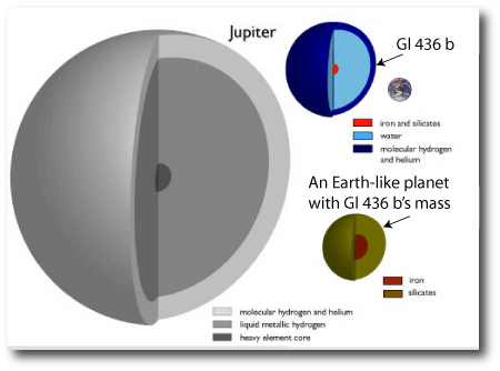
There’s a large difference in radius between sub-Neptune-mass planets made from rock and iron and sub-Neptunes composed mostly of water:

A Neptune transiting one of the brightest M-dwarfs in the sky would be a huge big deal. Hundreds of citations, Dude. Even if there’s no transit, this planet will likely be an excellent candidate for observation in the long-wavelength Spitzer bands, and fortunately there’s one more GO cycle before that cryogen runs out.

backlog

April 5, 2007

It was the end of the Winter quarter here at UCSC last week, and then I went on a trip, and then bam! More than a week with no posts… In the interim, there have been a number of interesting developments related to extrasolar planets. Here’s a brief run-down of some topics that I want to look at in more depth in the very near future:

Thanks to continuing efforts from the back-end user base, we’re accumulating a highly useful database of stable, low chi-square fits to the synthetic radial velocity data sets that comprise the Systemic Jr. catalog. Stefano has run a preliminary analysis and interpretation of the data. There are interesting implications for the overall eccentricity distribution of extrasolar planets, and there also appears to be a robust criterion for determining with confidence when you’ve extracted a real, previously unannounced planet from a given data set. We’re putting together a full report, which will appear quite soon. In the meantime, please keep submitting fits for systems that haven’t yet been adequately characterized.

The detection of another Neptune-mass planet orbiting a nearby red-dwarf was announced today. Yet more evidence for the core-accretion theory of planet formation! The discovery paper stops short of tabulating the radial velocities, but as I write this, Eugenio is busy dextering them onto the systemic back-end and onto the downloadable systemic console.

The theoretical case for the existence of Alpha Centauri B b is getting stronger by the day.

This year’s first ‘606 day is coming up next week, with a transit opportunity following on April 17th. I didn’t do enough to get the word out last December, but I’m hoping for good photometric coverage of the star during the upcoming window. A central transit for HD 80606b would last roughly 18 hours, so participation from observers worldwide will be required to definitively rule out transits.

Systemic Jr. Fit Drive

March 24, 2007

A big thank-you to everyone who’s been participating in the drive to characterize and study the catalog of synthetic “Systemic Jr.” planetary systems on the Systemic Backend. There’s now enough data to indicate that the analysis is going to be very informative. We’re looking forward to revealing the properties of the underlying planetary systems that were used to generate the data. In the meantime, we need your help to adequately characterize all 520 systems. Data in need of better characterization are marked by flags:

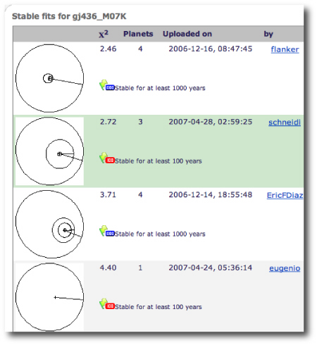
Our backend server is now swarming with various hard-working software robots that Stefano has assembled. The 100-year stability bot is rousted out of bed and set to work whenever a new fit is submitted. It reports a quick initial assessment of orbital stability. Planetary systems that pass through the 100-year stability screen are then put in a queue to wait for the attentions of the 1000-year stability bots. Systems that make it through 1000 years with less than a 1% change in semi-major axis of their planets are awarded a snazzy green flag:

Occasionally, systems that are in mean-motion resonance can show periodic semi-major axis variations of more than 1% while still remaining indefinitely stable. A resonance bot that will go through the fits and check for these special cases is currently being readied.

Systems that pass the minimum stability requirement are handed to a bootstrap bot which uses the bootstrap method to estimate uncertainties on the planetary orbital parameters for each stable fit. We’re currently running the bootstrap bot under the assumption that the orbits are pure Keplerian ellipses, and so the calculations are usually quite rapid. Very shortly, the error estimates for the parameters in submitted fits to the real systems and the Systemic Jr. systems will be showing up on the back-end data pages.

Finally, an “F-bot” has been activated which performs successive F-tests on submitted multiple-planet systems. Using its results, we’ll have a better idea of when the addition of a planet to a system is warranted.

HD 118206…

March 18, 2007

Most hot Jupiters have orbital eccentricities near zero because the tidal forces exerted on them by their parent stars are strong enough to rapidly circularize their orbits. Any planet whose orbit has been circularized should also be spin-synchronous, and so like our Moon with respect to the Earth, it should turn on its axis once every trip around the star. Synchronicity lends each hot Jupiter a permanent day and night side. This likely imparts a profound effect on both the planetary weather, and on the brightness of the planet when viewed in the infrared at different orbital phases.

All of the planets observed so far with the Spitzer Space telescope have nearly circular orbits, and hence are in (or are very near) the spin-synchronous state. We’re waiting to hear the results of our Spitzer GO-4 application to observe the highly eccentric planet HD 80606b, during an upcoming ‘606 day. If our observing proposal gets a thumbs-up, it’ll dramatically broaden the range of conditions under which planets have been observed. Very shortly, I’ll be posting the results of calculations that Jonathan Langton and I have been doing which predict what the light curve of HD 80606 should look like during the periastron passage in the various Spitzer bands. Here’s a sneak preview of how the temperature distribution on the planet might evolve over a 36-hour period as seen from a direction consistent with our line of sight from the Earth:

In looking over the latest officially published additions to the catalog of extrasolar planets, I noticed that there’s a very interesting object — HD 118203b — that straddles the extremes of the circular hot Jupiters and the ultra-eccentric HD 80606b. This planet was discovered in 2005 by the Swiss Team, has an orbital period of 6.13 days, a mass at least twice that of Jupiter, and a well-determined eccentricity, e=0.3. HD 118203b therefore won’t be spin-synchronous. Rather, as is also the case with HD 80606b (see the diagram here), it’ll have been forced into a state of pseudo-synchronous rotation, in which it does its best to keep one face toward the star during the periastron passage. Its day should be 64.8% as long as its year:

Which raises a rather interesting question: Why is HD 118203’s eccentricity so high?

Assuming that the planet has a similar structure to Jupiter, the equations of tidal dissipation (see here for a discussion) indicate that the planet’s orbit should circularize in a mere 10-20 million years. This time scale is surprisingly short because the parent star is a subgiant with a radius ~1.5 times larger than the Sun. Something must be exerting a very strong perturbation to keep this planet’s e up.

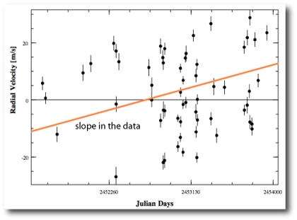
In their discovery paper, Da Silva et al remark that the residuals around the best 1-planet Keplerian fit to the data are very large. It’s quite straightforward to verify this with the downloadable Systemic console (try it!) Da Silva and company were able to improve their fit by including a linear drift of 49.7 meters per second with their one-planet model. This corresponds to adding the effect of an outer planet that has been observed for only a small part of a single orbit. (The 43 published velocities span a period of 1.1 years.) They speculate that an outer as-yet-uncharacterized planet provides the gravitational perturbation that maintains the high eccentricity for the inner planet.

Last year, Fred Adams and I wrote a computer code (see these papers 1, 2) that includes the effect of general relativistic corrections on long-term planet-planet gravitational interactions. It’s easy to use this program to calculate what the long-term influences of various companion planets would have on HD 118203 b’s eccentricity. I ran a few trial cases, and quickly found that the interactions produced by companions that also provide the observed linear drift in the radial velocities don’t seem to be strong enough to explain HD 118203b’s high eccentricity. Could there be another explanation?

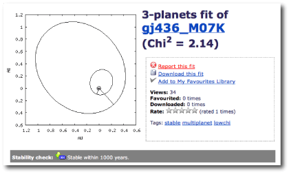
This is the sort of situation where the collaborative systemic back-end is extremely useful. I had a look at the stable fits that have been submitted so far for HD 118203. The best stable, self-consistent fit was uploaded back in October by the user Flanker, and has a reduced chi-square statistic of 1.96:

null .

This fit might point in an interesting direction for some further inquiry. Instead of using a linear trend to soak up the residuals to the one-planet fit, Flanker added two additional planets. One of the planets has a mass of 0.3 Jupiter masses and is orbiting with a period of 15 days. Its periapse is nearly aligned with the periapse of the inner planet. The resulting short-period secular interaction may well be strong enough to keep the eccentricity of the innermost planet high in the face of tidal dissipation. Flanker’s model also contains an outer planet with an orbital period of 244 days and a minimum mass 0.6 times that of Jupiter.

I think it’s worthwhile to explore additional models for this system that contain planets with short enough periods to intereact strongly with the 6.13 day planet. If the perturbing body has a relatively short-period orbit, then its presence will not be hard to verify with additional radial velocity observations of the star. And also, if Spitzer’s cryogen holds out, HD 118203b might be a very interesting target for a full-phase campaign.

Bootstrap

March 10, 2007

Stefano and Eugenio have been making quite a bit of development progress on the downloadable systemic console. A new version of the console (available for beta testing on the systemic backend) is now capable of providing an estimate of the uncertainties on the orbital elements associated with a fit to a particular data set.

Radial velocity data don’t provide an exact determination of planetary orbits. The most obvious shortcoming is that Keplerian orbital fits can’t determine the inclination of the planetary orbits, and so for a given system, we’re only able to measure then mass of the planet multiplied by the sine of the unknown inclination angle. Furthermore, the stellar radial velocity signal created by a planetary system is corrupted by astrophysical noise introduced by the parent star, as well as by noise introduced during the measurement process here on Earth.

Determination of the true uncertainties in a planetary orbital model is a subtle problem (for more detail, see Eric Ford‘s recent work in this area). As a first straightforward step, we’ve implemented the so-called “bootstrap” method of error estimation into the console. The bootstrap works by taking the original data set, and then successively redrawing time + velocity + uncertainties triples from the data with replacement. This procedure creates alternate realizations of the original data set in which some of the original measurements appear more than once, and in which some don’t appear at all. The best-fit parameters obtained by the console are then used as a starting guess to fit the bootstraped data sets. The standard deviations measured from the distributions of orbital elements thus obtained give error estimates for the parameters of the original fit.

The bootstrap routine is menu-accessed, and is simple to use. First, create a fit to a dataset. In the example just below, I’ve fitted to the data for HD 80606:

Once the fit has been polished, the bootstrap can be run. In the default configuration it uses Keplerian fitting and does 100 trials.

HD 80606 has been observed for nearly 20 orbital periods, and velocities have been obtained at a wide variety of orbital phases. As a result, the orbit is very well constrained. The bootstrap indicates that the uncertainty on the e=0.932 eccentricity is only 0.003. For other systems, such as hd 20782, which also seems to have a high eccentricity:

the uncertainty on the parameters is much larger:

Give the routine a try! In upcoming posts, we’ll talk more about how uncertainty estimates will be incorporated into the planetary catalogs on the backend.

Impact!

March 7, 2007

The news out of the Planetary Defense Conference is that NASA has the ability to locate all the potentially dangerous asteroids in our solar system by the year 2020, but that the cash to carry out the project is not currently forthcoming.

CNN and many other news outlets carried the story, along with a dramatic artist’s rendition of an asteroid striking the Earth.

That’s a rather large asteroid.

Measuring the circumscribed circles, it appears that the impacting body is 1/10th the Earth’s diameter, or approximately 600 km in radius. A bolide of this magnitude would currently rank as the ~25th largest object in the solar system, larger than Uranus’s moon Umbriel (584 km radius), smaller than Saturn’s moon Iapetus (736 km in radius), and nearly exactly the same size as Pluto’s moon Charon (606 km in radius). Ceres, the largest object in the main asteroid belt, by contrast, has a radius of ~475 km.

Based on the location of the late-afternoon catastrophe relative to the day-night terminator, the impactor seems to have had an orbit that was highly inclined relative to the solar system’s angular momentum plane. Perhaps it was undergoing Jupiter-driven Kozai oscillations prior to striking the Earth.

The last impact of the magnitude shown in the illustration was probably the Moon-forming impact ~4.4 Billion years ago, in which a Mars-sized body struck the Earth. Kevin Zahnle of the NASA Ames Research Center has estimated the distribution of giant impacts after the Moon-forming event. It’s likely that the largest strikes were by bodies with roughly half the radius of the object shown in the above picture.

The consequences of even a 300 km object hitting the Earth are severe. Such an impact is energetic enough to entirely vaporize the Earth’s oceans and create a temporary rock-vapor atmosphere with a surface pressure of ~100 bars. For a period of several months to a few years, the Earth would radiate with a temperature of ~2000 Kelvin — hot enough to glow brightly in the visible region of the spectrum. And depressingly, our planet would be fully sterilized by the event.

This week’s crop

March 6, 2007

Image Source.

The year 2007 is off to a reasonably good start. Three more planets were announced by the Geneva Planet Search team at a conference in Chile, bringing the total planet crop for ’07 up to seven.

The rate of planet discovery, however, has definitely leveled off. For the past four years, the detection rate has remained fixed at 26 new planets per year. The low-hanging fruit — the 51 Pegs, the 47 Ursae Majorii, the Upsilon Andromedaes — have all been harvested from the bright nearby stars, and increasingly extractive methods are being brought to bear. Transits are starting to contribute significantly to the overall detection rate. Radial velocity is pushing to planets with progressively lower masses. Surveys such as N2K are rapidly screening metal-rich stars that have high a-priori probabilities for harboring readily detectable planets. The neccessity of finding more planets is driving up the average metallicity of the known planet-bearing stars:

The three new planets, HD 100777b, HD 190647b, and HD 221287b are quite ordinary as far as extrasolar planets go. They all have masses somewhat greater than Jupiter, and they all take more than a year to orbit their parent stars. Their discovery seems not to have registered with the news media:

HD 100777 b, however, is actually deserving of some attention. Its orbital period of 383.7 days places it squarely in the habitable zone of its parent star. The eccentricity, e=0.36, is fairly high, and likely leads to interesting seasonal effects in the atmosphere of the planet.

HD 100777 b lies a regime where we expect to see white water clouds forming in the visible atmosphere. The planet is probably very reflective in the optical region of the spectrum (quite unlike the hot Jupiters, which are likely cloud-free, and which are known to absorb almost all of the starlight that strikes them). Convection of interior heat to the surface of HD 100777b is almost certainly driving collossal thunderstorms, and the atmospheric disturbances created by the thunderstorms likely feed giant vortical storms similar to Jupiter’s great red spot.

It’s also possible that the atmosphere is much clearer in regions where air wrung dry by rainfall is downwelling. This phenomenon occurs on Jupiter, where highly transparent patches occur over several percent of the Jovian surface:

The Galileo entry probe went right into one of these regions, and sampled very dry air. On HD 100777, the regions of high atmospheric transparency will probably preferentially absorb red and green light (as a result of Rayleigh scattering of incoming photons). The surface, then, in the vicinity of a downwelling region may look something like this: