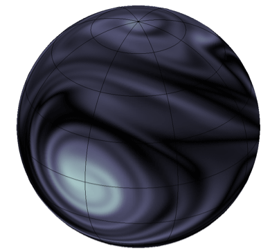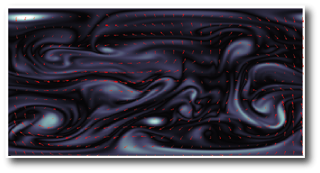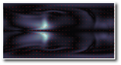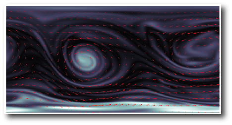
Vorticity

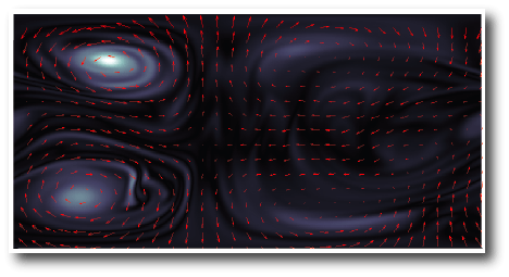
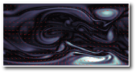
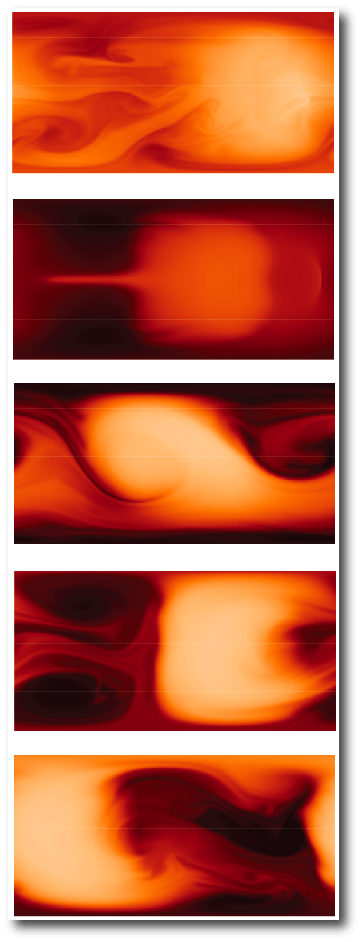
Vorticity can be thought of as the tendency of a paddlewheel to spin if placed in the flow. High vorticity is a large counter-clockwise spin, zero vorticity is no spin, and a large negative vorticity is a tendency to spin clockwise. The climate models of short-period extrasolar planets that Jonathan Langton and I have developed show a remarkable variety of vorticity patterns on their surfaces, in keeping with the incredibly stormy and complex nature of their atmospheres. Here’s a gallery of Mercator-projection vorticity maps for the known strongly irradiated Jovian planets that have significant eccentricities. The red arrows indicate the wind speeds and directions across the planetary surfaces. These figures are all from a paper that’s currently under review at the Astrophysical Journal (see here for an overview of the numerical method that we’re using). Also, a shout-out is due to Edward Tufte for advocating the strong graphic-design effect of small spots of saturated color on a gray-scaled backdrop.


HAT-P-2b
:

Here are 1.1 MB North Pole, South Pole and Mercator Projection animations of the HAT-P2b vorticity evolution.

HD 80606 b
:

1.1 MB Mercator animation here.

HD 185269 b:

1.1 MB Mercator animation here.

HD 108147 b

1.1 MB Mercator animation here.

HD 118203 b
:

1.1 MB Mercator animation here. The animations above are hosted on the Oklo Corporation’s servers.

It’s interesting to compare the vorticity maps with the temperature distributions on the planetary surfaces (shown in the same order as above):

Gigantic

Image Source.

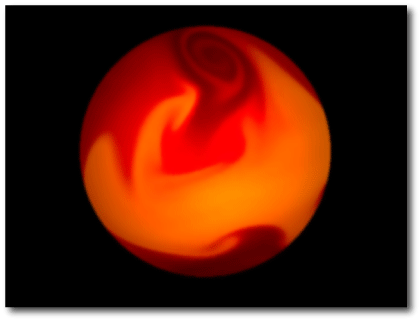
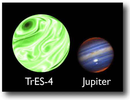
The TrES survey announced the discovery of a new transiting planet today, raising the number of known transits to twenty (including Mercury and Venus). The new planet, “TrES-4”, has a mass of order 84% that of Jupiter, and with a radius of 1.67 Rjup, it’s pumped to nearly five times Jupiter’s volume:

The false color image of Jupiter was produced from near-infrared data obtained with the Gemini telescope. The even more luridly false-color representation of TrES-4 is based on a vorticity map from one of Jonathan Langton’s recent simulations.

In order for TrES-4 to be swollen to its current size, it needs to be experiencing heating of order 6×10^27 ergs per second. One way to do this is to have a significant perturbing companion which drives large time-averaged variations in TrES-4’s orbital eccentricity. So far, there are only four published radial velocities for TrES-4, so the orbit could easily be non-circular. More provocatively, if strong orbital forcing is indeed occurring, then there’s a reasonable chance that the perturber might also be observable in transit. I recommend that Transitsearch.org observers keep this bad boy under constant supervision.

Whorls

Image Source.

HAT-P-2b. The name doesn’t exactly ring of grandeur, but this planet — a product of Gáspár Bakos’ HAT Net transit survey — is poised to give the Spitzer Space Telescope its most dramatic glimpse to date of a hot Jupiter.

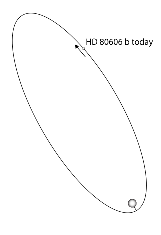
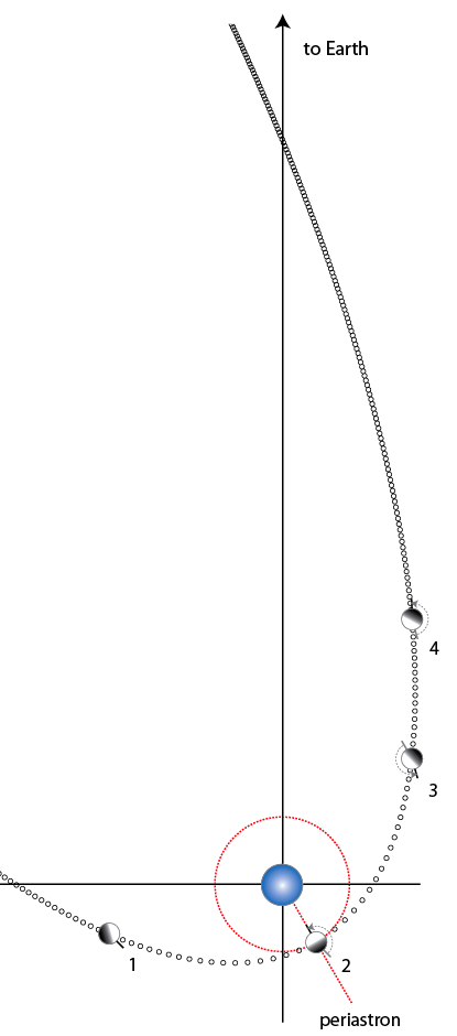
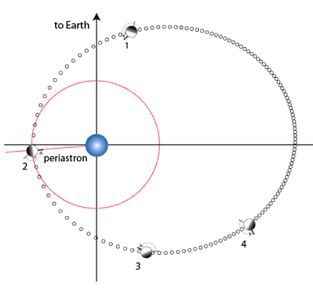
HAT-P-2b’s orbit is remarkably eccentric for a planet with an orbital period of only 5.6 days, and by a stroke of luck, periastron is located almost exactly midway between the primary and the secondary transits (as viewed from Earth). The strength of the stellar insolation at periastron is nine times as strong as at apastron, which more than guarantees that the planet will have disaster-movie-ready weather.

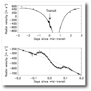
On June 6th, Josh Winn and his collaborators used the Keck telescope to obtain 97 radial velocities for HAT-P-2. The observations were timed to occur before, during, and after primary transit, and the Rossiter-McLaughlin effect is clearly visible in their data (preprint here):

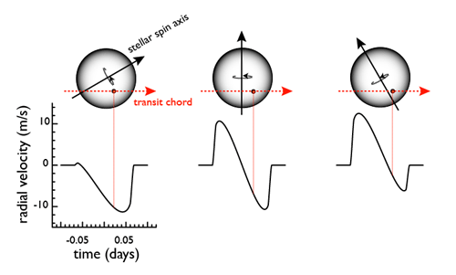
The symmetry of the Rossitered points indicates that the angular momentum vector of the planetary orbit is aligned with the spin pole of the star:

schematic diagram showing rossiter effect

This state of affairs also holds true for the other transiting planets — HD 209458b, HD 149026b, HD 189733b — for which the effect has been measured. The observed alignments are evidence in favor of disk migration as the mechanism for producing hot Jupiters.

With its apparent magnitude of V=8.7, the HAT-P-2b parent star is roughly ten times brighter than the average planet-bearing star discovered in a wide-field transit survey. The star is bright enough, in fact, to have earned an entry in both the Henry Draper Catalog (HD 147506) and the Hipparcos Database (HIP 80076), but with its surface temperature of 6300K (F8 spectral type) it was too hot to have been a sure-fire “add” to the ongoing radial velocity surveys. Prior to this May, it had been entirely ignored in the astronomical literature (save a brief mention in this paper from 1969).

HAT-P-2’s intrisic brightness and its planet’s orbital geometry mean that in a relatively compact 34-hour observation, Spitzer can collect on the most interesting features of the orbit with high signal-to-noise. In particular, there is an excellent opportunity to measure the rate at which the day-side atmosphere heats up during the close approach to the star. The planet, in fact, presents such a remarkable situation that a block of Director’s Discretionary time was awarded so that the observations can be made during the current GO-4 cycle. They’ll be occurring soon.

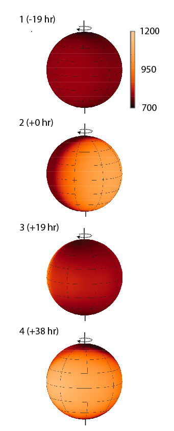
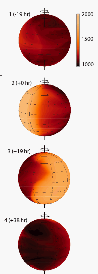
Both HAT-P-2b and HD 80606 b will provide a crucial ground truth for extrasolar planetary climate simulations. Jonathan Langton’s current model, for example, predicts that that the temperatures on HAT-P-2b will range over more than 1000K. At the four times shown in the above orbital diagram, the hemisphere facing Earth is predicted to show the following appearances:

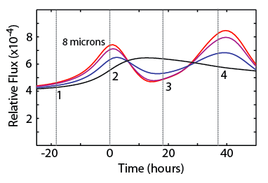
Spitzer, of course, can’t resolve the planetary disk. It measures the total amount of light coming from the planet in chosen passband. At 8-microns, the planet’s light curve should look like this:

The temperature maps only hint at the complex dynamics of the surface flow. A better indication is given by the distribution of vorticity,

which we’ll pick up in the next post…

Showing Mercury the Door (Part 1).

The long-term stability of the planetary orbits has been a marquee-level question in astronomy for more than three centuries. Newton saw the ordered structure of the solar system as proof positive of a benign deity. In the late 1700s, the apparent clockwork regularity of interaction between Jupiter and Saturn helped to establish the long-standing concept of Laplacian determinism. In the late Nineteenth Century, Poincaré’s work on orbital dynamics provided the first major results in the study of chaotic systems and nonlinear dynamics, and began the tilt of the scientific worldview away from determinism and toward a probabalistic interpretation.

In the past ten years, it has become fairly clear that the Solar System is dynamically unstable, in the sense that if one waits long enough (and ignores drastic overall changes such as those wrought by the Sun’s evolution or by close encounters with passing stars) the planets will eventually find themselves on crossing orbits, leading to close encounters, ejections and collisions. The question has shifted more to the following: What (if any) chance is there that the planets will experience orbit crossings within the next 5 billion years?

It’s clear that the probability of the planets going haywire prior to the Sun’s red giant phase is pretty small. Computers are now fast enough to integrate the eight planets forward for time scales of ten billion years or more. Konstantin Batygin, a UCSC physics undergrad who has been collaborating with me, has been running a suite of very long term solar system integrations, and he’s been getting some nice results.

It’s well known that over the long term, the planetary orbits are chaotic. The Lyapunov timescales for the planetary orbits in both the inner and the outer solar system are of order a few million years, which means that for durations longer than ~50 Myr into the future, it becomes impossible to make a deterministic prediction for exactly where the planets will be. . We have no idea whether January 1, 100,000,000 AD will occur in the winter or in the summer. We can’t even say with complete certainty that Earth will be orbiting the Sun at all on that date.

We can, however, carry out numerical integrations of the planetary motions. If the integration is carried out to sufficient numerical accuracy, and starts with the current orbital configuration of the planets, then we have a possible future trajectory for the solar system. An ensemble of integrations, in which each instance is carried out with an unobservably tiny perturbation to the initial conditions, can give a statistical distribution of possible long-term outcomes.

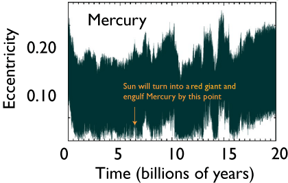
Here’s a time series showing the variation in Earth’s eccentricity during a 20 billion year integration. In this simulation, the Earth experiences a seemingly endless series of secular variations between e=0 and e=0.07 (with a very slight change in behavior at a time about 10 billion years from now). The boring, mildly chaotic variations in Earth’s orbit are mostly dictated by interactions with Venus.

Mercury, on the other hand, is a little more high-strung.

These two plots suggest that the Solar System is “good to go” for the foreseeable future. Indeed, work by Norm Murray and Matt Holman suggests that the four outer planets have a dynamical lifetime of order one hundred quadrillion years. Work by Jaques Laskar, however, suggests that the inner solar system might be on far less stable footing. Konstantin has obtained some very interesting new results on this particular point, which we’ll be sharing in an upcoming post…

HAT-P-3b

Image Source.

The HATNet survey’s latest single, “3b” landed on the charts last week at #12. This hot (Teff~1053K) new disk shows a definite metal influence, which makes sense, given that [Fe/H] for the parent star is an Ozzy-esque +0.27. You can get a free download of the paper from the Extrasolar Planets Encyclopaedia.

The past twelve months has seen the inventory of known transiting planets more than double, as wide-field surveys such as TrES, Exo, and HATnet start to reach the full production end of their observational pipelines. As the number of planets reaches the threshold for statistical comparisons, interesting trends (or possible trends) have started to emerge.

By far the most remarkable correlation, however, has been with respect to sky location. Among the fourteen fully announced transiting planets orbiting stars with V<14, every single one is located north of the celestial equator.

Planet

Mass

Mjup

Period

days

Dec V
Gl 436b 0.07 2.64385 +26 42 10.68
HAT-P-1 b 0.53 4.46529 +38 40 10.4
HAT-P-3 b 0.61 2.8999 +48 02 11.86
HAT-P-2 b 8.64 5.63341 +41 03 8.71
HD 149026 b 0.36 2.8766 +38 21 8.15
HD 189733 b 1.15 2.21857 +22 43 7.67
HD 209458 b 0.69 3.52475 +18 53 7.65
TrES-1 0.61 3.03007 +36 38 11.79
TrES-2 1.98 2.4703 +49 19 11.41
TrES-3 1.92 1.30619 +37 33 12.4
WASP-1 b 0.89 2.51997 +31 59 11.79
WASP-2 b 0.88 2.152226 +06 26 11.98
XO-1 b 0.9 3.941534 +28 10 11.3
XO-2 b 0.57 2.615838 +50 13 11.18

Looks like there’s some opportunity down under…

Barred Spiral

Image Source.

I’d never really seen the Milky Way until I saw it on a perfectly clear and moonless July night from a spot just below the Arc Dome in central Nevada. It spills a swath of patchy luminosity that seems to split the sky in half; a barred spiral galaxy, seen edge-on, and from within. One hundred billion intensely glowing stars, like sand grain jewels, each separated by miles. The photo above (taken by Steve Jurvetson last weekend from the Black Rock Desert in Nevada) reminded me of that experience.

The dark sky applet shows that the interior of Nevada (away from Las Vegas!) contains many of the least light-polluted areas of the United States.

Under a totally dark sky, you can distinctly see the star clouds in the foreground of the galactic center. It’s eerie to think that the 3-million solar mass black hole lurking in the center of the galaxy is just to the right of the bright luminosity of Baade’s Window near the boundary between Sagittarius and Scorpius.

The photo also shows Jupiter within a few degrees of Antares — a nice illustration of the fact that Jupiter appears slightly brighter than the brightest stars.

Newton used this similarity in apparent brightness to get the first real estimate of the staggering distances to the stars. He assumed that the stars are similar in absolute brightness to the sun, and he assumed that Jupiter (whose distance and angular size were known to him) is a perfect reflector of sunlight. This method underestimates the distance to Sirius by more than a factor of five, but it does a fairly reasonable job for Alpha Centauri.

A hot hot Neptune

Image Source.

Regular oklo readers will recall Gillon et al.’s discovery that the Neptune-mass planet orbiting the red dwarf star Gl 436 can be observed in transit. Transitsearch got scooped, and the whole eposide got me all worked up enough to neglect the exigencies of everyday academic life and reel off three straight posts on the detection and its consequences (see here, here, here, and also here). The transits of Gl 436 b are a big deal because they indicate that the planet is possibly composed largely of water. It’s not a bare rock and it’s not a Jupiter-like gas giant. Rather, it’s consistent with being a fully Neptune-like object, hauled in for inspection on a 2.64385 day orbit.

Following Gillon et al.’s announcement, it became clear that Gl 436 transits would fit into a window of observability during the June 24th – July 04 IRAC campaign on the Spitzer Space Telescope. The red dwarf parent star, furthermore, because of its proximity, is bright enough for Spitzer to achieve good photometric signal-to-noise at 8-microns. As a result, Joe Harrington’s Spitzer Target of Opportunity GO-4 proposal was triggered, and the Deep Space Network radioed instructions to the spacecraft to observe the primary transit on June 29th, as well as the secondary eclipse (when the planet passes behind the star) on June 30th, a bit more than half an orbit later. Joe, along with his students Sarah Navarro and William Bowman, and collaborators Drake Deming, Sara Seager, and Karen Horning asked me if I wanted to participate in the analysis. After watching all the ‘436 action from the sidelines in May, I was more than happy to sign up!

One of the most exciting aspects of being a scientist is the round-the-clock push to get a time-sensitive result in shape for publication. There’s a fantastic sense of camaraderie as e-mails, calculations, figures and drafts fly back and forth. On Monday afternoon PDT (shortly after midnight GMT) when Mike Valdez sent out his daily astro-ph summary, it was suddenly clear that we were under tremendous pressure to get our results analyzed and submitted. The Geneva team had swooped in and downloaded the data for the primary transit the moment it was released to the community! They had cranked out a reduction, an analysis, and a paper, all within 48 hours. Their light curve confirmed the ground-based observations. Spitzer’s high-quality photometry indicates that the planet is slightly larger than had been indicated by the ground-based transit observations. Drake submitted our paper yesterday afternoon.

Fortunately for us, the real prize from Spitzer is the secondary eclipse. Its timing is capable of independently confirming that the orbit is eccentric, and the depth gives an indication of the surface temperature on the planet itself.

The upper panel of the following figure shows the raw Spitzer photometry during the secondary eclipse window. IRAC photometry at 8 μm is known to exhibit a gradually increasing ramp-up in sensitivity, due to filling of charge traps in the detectors, but even before this effect is modeled and subtracted, the secondary transit is visible to the eye. The bottom panel shows the secondary transit in detail.

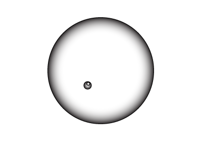
The secondary transit occurs 58.7% of an orbit later than the primary transit, which proves that the orbit is eccentric. A detailed fit to the transit times and to the radial velocities indicates that the orbital eccentricity is e=0.15 — halfway between that of Mars (e=0.1) and Mercury (e=0.2). The orbital geometry can be drawn to scale in a diagram that’s 440 pixels across:

The depth of the secondary eclipse is 0.057%, which allowed us to estimate a 712 ± 36K temperature for the planetary surface.

A temperature of 700+ K is hotter than expected. If we assume that the planet absorbs all the energy that it gets from the star and re-radiates its heat uniformly from the entire planetary surface, then the temperature should be T = 642 K. The higher temperature implied by the secondary eclipse depth could arise from inefficient transport of heat to the night side of the planet, from a non-“blackbody” planetary emission spectrum, from tidal heating, or from a combination of the three. If the excess heat is all coming from tidal dissipation, then the Q-value for the planet is 7000, suggesting that it’s a bit more dissipative inside than Uranus and Neptune.

What would Gl 436 b look like if we could go there? To dark adapted eyes, the night side is just barely hot enough to produce a faint reddish glow (as is the case on the surface of Venus, which has a similar temperature). The atmosphere is too hot for water clouds, and is likely transparent down to a fairly high atmospheric pressure level. The day-side probably reflects a #E0B0FF-colored hue that contrasts with the orange-yellow light of the star. The planet spins with a period of 2.32 days so that it can be as spin-synchronous as possible during the sector of its orbit closest to periastron. At a fixed longitude on the planet, the day drags on for 456 hours from high noon to high noon.

Jonathan Langton has been running atmospheric simulations with the latest parameters. On the phone, just a bit ago, he would only say that the preliminary results were “interesting”…

Second quarter earnings report

Image Source.

On Thursday and Friday of last week, the Dow Jones Industrial Average jumped nearly 2%. Given the soaring price of oil and the subprime mortgage crisis, many students of the financial markets were puzzled by this seeming burst of irrational exuberance.

A visit to exoplanet.eu, however, suggests that investors and speculators were placing buy orders in response to the rapid recent increase in the number of known planets. During the first two quarters of ’07, the extrasolar planet detection rate has been running more that 100% above the rate reported for the most recent full fiscal year.

When asked about the impact of the new discoveries, one metals trader was quoted, “Well, Mate, the Marketplace has been pricing in the core-accretion theory for several years now. That means we’re looking at a Z of ~0.1 for each one of these planets coming in, so that’s roughly 30 Earth masses of ore per extrasolar planet. If we use the solar gold assay, that works out to one quintillion ounces of new proven reserves for each discovery. With gold at $660, we’re starting to talk real money.”

Jocularity aside, the raft of new planet discoveries is having a noticeable impact on the correlation diagrams that can be explored at the exoplanets.eu site. One (likely statistically insignificant) curiosity is the lack of Saturn-mass planets in this year’s crop to date. At the low-mass end, Neptunes such as Gl 674b are turning up with increasing frequency, and the detection-rate for Jupiter-mass planets and above also remains strong. This dichotomy is very much in line with a key prediction of core-accretion in its simplest form. The rapid gas accretion that occurs once the planet mass reaches ~30 Earth masses should tend to make Saturn-mass planets relatively rare.

Another interesting diagram results when one plots the masses and eccentricities of the known RV-detected planets. A glance at the resulting diagram indicates that low-mass planets tend to be on more circular orbits. Could this be hinting at two populations of planets and (perhaps) two different formation mechanisms? It’s hard to tell. Much of the effect comes from the fact that low-mass planets need to have short periods in order to be detectable. Short-period planets, in turn, are far more affected by tidal circularization of the orbits. The plot is also reflecting the still-mysterious (but well known) shortage of high-mass hot Jupiters.
GJ 876 d

Image Source.
Galileo’s discovery of the four major Jovian satellites — his Medicean Stars — revealed that Jupiter is accompanied by a planetary system in miniature. In his Dialogue on the Two Chief World Systems, Galileo drew on the obvious analogy between Jupiter and its moons on the one hand and the Sun and the planets on the other as evidence in favor of the Copernican worldview.

The pattern is that when an orbit is larger, the revolution is completed in a longer period of time; and when smaller, in a shorter period. Thus Saturn, which traces a greater circle than any other planet, completes it in thirty years; Mars in two; the moon goes through its much smaller orbit in just a month; and in regard to the Medicean stars, we see no less sensibly that the one nearest Jupiter completes its revolution in a very short time (namely about forty-two hours), the next one in three and one-half days, the third one in seven days, and the most remote one in sixteen. This very harmonious pattern is not changed in the least as long as the motion of twenty four hours is attributed to the terrestrial globe (rotating on itself).

Image Source.

Two decades ago, prior to the discovery of the extrasolar planets, the Galilean satellites, along with the regular satellite systems of Saturn and Uranus, constituted one of the strongest hints that extrasolar planets should exist. In each case, the total fractional mass and relative orbital scale of the satellites is quite similar, implying that a robust and generic formation process was at work. There’s a factor-of-twenty difference between the masses of Jupiter and Uranus, but the fractional mass caught up in their satellites differs by only a factor of two. The Jovian satellites add up to 0.021% of Jupiter’s mass, whereas the Uranian moons amount to 0.011% of Uranus’ mass. Similarly, the Saturnian satellite system (which is completely dominated by Titan) has a total mass amounting to 0.025% of Saturn. In all three cases, the orbital distance of the outermost large satellite is between 20 and 60 planetary radii.

Robin Canup and Bill Ward of Boulder’s Southwest Research Institute have developed a compelling formation model that naturally accounts for the similarities between the giant planet satellite systems (see here and here). In their picture, regular satellites build up from solid particles that flow into the circumplanetary disks from the surrounding solar nebula. Once a nascent moon reaches a non-trivial size, it decouples from the inward spiral of gas, and is able to rapidly accrete large quantities of solid particles. Ultimately, a satellite’s ability to grow to very large size is shuttered by Type I migration, whose timescale decreases in inverse proportion to the satellite mass. In the Canup-Ward picture, a succession of Jovian satellites form and are accreted onto the central planet when their mass exceeds ~0.02% of the planetary mass.

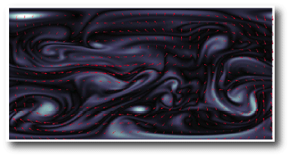
The flow pattern in the outer region of a protoplanet’s Roche lobe that regulates the flow of gas into the circumplanetary disk is quite complicated. Here’s an image adapted from the hydrodynamical simulations of Steve Lubow and his collaborators (paper here) that shows the streamlines in the vicinity of the forming planet’s Roche lobe:

The gravity of the Sun produces a tidal barrier which meters the flow of gas into the protoplanetary disk, and Canup and Ward compare the Jovian satellites to the buildup of mineral deposits on the interior of a pipe through which a great deal of water has flowed.

Squeezing out regular oklo posts is a bit of a challenge. I want to keep the posting schedule fairly regular in order to keep the readership up, but at the same time, its sometimes hard to keep coming up with post-worthy topics. In trolling for ideas, I often go to the Extrasolar Planets Encyclopaedia and comb through the tables, looking for patterns or analogies. A bit more than a year ago, I noticed that Gl 876 d, with its 1.92-day orbit and its 0.007% mass ratio is reminiscent of a Jovian satellite. Could it have arisen from a direct analog of the Canup-Ward formation process?

In the Gl 876 system, the middle planet c would have metered the gas flow into Gl 876’s inner circumstellar disk. A considerable amount of the inward flowing gas in the nascent Gl 876 system would have accreted onto planet c, but there was likely a stream (or streams, given the additional presence of planet b) that bypassed the planets and flowed onto the inner disk. The low density of steadily flowing gas in the inner disk would have allowed planet d to feed on the incoming solid material while staving off demise via Type I migration. The formation of d through this process would have occurred entirely within the Gl 876 snowline, and so in this picture, planet d is composed largely of iron and silicates. Figure 10 from the Lubow et al. paper gives a nice sense of how gas and small solid particles would have slipped by planet c on their way in:

Willy Kley and his collaborators have done hydrodynamical simulations which model the interaction between that the outer two Gl 876 planets and the parent gas disk. The flow pattern in the vicinity of the planets is more complicated than in the single-planet case, and streams of gas (and small particles) are able to flow into the disk region interior to the 30-day orbit of planet c. It’s not unreasonable to imagine that the combined presence of planets b and c mediated an inner circumstellar disk around GJ 876 that was reminiscent of the circumplanetary disk around a Jovian planet. Here’s an example figure from the Kley et al. paper showing the hydrodynamical flow in the vicinity of planets b and c:

It thus seems plausible that GJ 876 d could indeed owe its origin to the same process that produced the Jovian satellites. The planet d that shows up in the radial velocity data might be the largest survivor among a number of similar iron-silicate planets that formed in the gas-starved inner disk and were then lost to the star via type I migration. In keeping with the analogy to Jovian satellites, this scenario would hint at additional, somewhat smaller iron-silicate planets circling Gl 876 in orbits with periods in the 4-12 day range. Looks like more RVs are in order!

A manufacturing scheme akin to the giant planet satellite formation process is, however, not the only way to produce Gl 876 d. Doug Lin and his collaborators, for example, have suggested that GJ 876 d formed from pre-existing icy planetesimals that were herded inward during the resonant migration of the massive outer planets b and c. In their picture, Gl 876 d is made largely from water, and would thus have a larger physical radius than if it was built primarily from silicates via a Jovian satellite-like formation process. Mandell et al. outline a related mechanism by which d could have formed via resonant shepherding.

It’s a shame that d doesn’t transit.

Are there any other inner planets that might be candidates for formation via the Canup-Ward mechanism? Plausible clues would consist of a short orbital period, a ~0.01% mass ratio, and a massive outer planet in a ~10-50 day orbit. 55 Cancri e just might fit that bill…

planeticity vs. metallicity

Image Source.

Mike Valdez pointed me to an interesting paper by Pasquini et al. that was posted to astro-ph today. The authors examined the frequency with which Jovian-mass planets are detected around giant stars and dwarf (that is, ordinary main sequence) stars as a function of the metallicity of the host star. Their main result is summed up in this redrawn figure:

The red histogram shows the well-known result that detectable Jovian-mass planets are preferentially found around metal-rich stars. The blue histogram shows a result that seems surprising at first glance. It indicates that for giant stars, the metallicity effect essentially goes away. The distribution in the blue histogram is not much different from the overall distribution of stellar metallicities in our local galactic neighborhood.

Pasquini et al. give several possible explanations for their result. Their favored interpretation is that the planet-metallicity correlation is due not to high intrinsic metallicity, but rather to stellar pollution. The idea is that after a planet-bearing star forms, its thin convective envelope is enriched by the accretion of heavy elements. The planet-bearing stars that have metal-rich spectra are in actuality ordinary stars sheathed in enriched envelopes. As polluted stars evolve off the main sequence, their convective envelopes grow deeper, and the apparent metallicity enhancements largely disappear.

As an inveterate adherent of the core-accretion hypothesis for the bulk of giant planet formation, my knee-jerk reaction is to be unhappy with a pollution interpretation. Disks and (by extension) stars that are metal-rich are more capable of building planetary cores while there’s still gas remaining in the protoplanetary disk. The planet-metallicity connection is thus a natural consequence of the core accretion hypothesis.

Pasquini et al. point out that the giant stars in their sample are systematically more massive than the main-sequence stars for which the planet-metallicity connection has been established. This leads them to speculate:

Since the fraction of planet-hosting giants is basically independent of metallicity, it is feasible that intermediate mass stars favor a planet formation mechanism, such as gravitational instability, which is independent of metallicity. One could speculate that such a mechanism is more efficient in more massive stars, which (likely) have more massive disks.

I don’t completely agree with this interpretation either, but I do think that the correct explanation is tied into a systematic difference in stellar mass between the giant sample and the dwarf sample. While it’s somewhat difficult to get accurate masses for giants, its reasonable to assume that the average mass of the giants in the above histogram is ~2 solar masses. If we assume that protostellar disks scale in mass with the mass of the parent star, then the average disk around a 2 solar mass star had roughly twice the surface density of solids than the average disk around a solar mass star. This is equivalent to a 0.3 dex increase in metallicity in a disk around a solar mass star, neatly explaining the magnitude of the offset between the red and the blue histograms.

The paucity of planets around high-metallicity giants probably stems in part from small number statistics and from the fact that there are very few super-metal-rich giants in the survey. Note that the histograms plot the distributions in metallicity for planet-bearing stars, and not the fraction of planet-bearing stars in a complete sample as a function of metallicity Although a detailed Monte-Carlo experiment is definitely in order, I think that Pasquini et al.’s result will end up being fully in line with the expectations of the core-accretion theory.

This argument would have had a lot more weight if I’d done a detailed Monte-Carlo analysis in advance, rather than monday-morning-armchair-quarterbacking (that is, blogging) with a smug postdiction. I think, however, that the core-accretion theory indicates that these general trends will all continue to hold true:

N equals L

Image Source.

Last weekend, I participated in the “Future of Intelligence in the Cosmos” workshop at NASA Ames. In an age of ultra-specialized conferences, the focus for this one bucked the trend by pulling back for the really big picture:

The Future of Intelligence in the Cosmos” is an interdisciplinary two-day workshop that seeks to elucidate potential scenarios for the evolution of intelligent civilizations in our galaxy and thus, perhaps, to find a resolution for this seeming paradox. The probability that intelligent civilizations exist has been succinctly stated by the Drake Equation. While the first few terms in the equation, such as the number of stars in the Milky Way Galaxy, the fraction of stars that have planets, and the number of planets in the habitable zone, are becoming better known, the last three terms that depict the fraction of planets that evolve intelligent life, the fraction that communicate, and the fraction of the lifetime of the Milky Way Galaxy over which they communicate, are not well known. It is these last three terms in the Drake Equation that are the focus of the workshop.

In most venues, extrasolar planets veer toward the esoteric. At this workshop, however, the galactic planetary census was perhaps the most nuts-and-bolts topic on the agenda. We know that planet formation is common in the galaxy, and its increasingly clear that the “great silence” isn’t stemming from a lack of Earth-mass worlds.

Here’s a link to a .pdf document containing the slides from my talk.

In an upcoming post, I’ll try to pull together a synopsis of what emerged from the conference. Perhaps the most startling moment for me came in Paul Davies‘ talk, when he described the extent to which the simulation argument has been developed.

When I was in graduate school, Frank Drake was a faculty member in our Department. I noticed right away that the license plate on his car read “neqlsl”. I always read this as “n equals one”, until I finally asked him which term was responsible for thwarting all the alien civilizations.

“It’s not N equals one,” he said, “it’s N equals L”.

A miss is as good as a mile

Image Source.

When I give a public lecture, I often start by trying to impart a sense of the extraordinarily rarefied character of the local galactic neighborhood. The known catalog of planet-bearing stars is akin to 200 small grains of sand dusting a volume more than 1000 kilometers on a side. It seems amazing to me that we’re able to see the stars at all with the naked eye. Even Sirius appears twelve billion times fainter than the Sun.

At the moment, the Alpha-Proxima trio is the closest group of stars to the Sun, and they are currently drawing closer still. In 27,000 years, they will pass at a minimum distance of 2.75 light years. Already, the Alpha-Proxima system is beginning to have an effect on the Oort Cloud, and as a result of the encounter, roughly half a million comets will be delivered into Earth-crossing orbits over the next several million years. This will generate something like a 10% increase in the arrival of new comets above the long-term average.

In 1999, Joan Garcia-Sanchez and collaborators filtered the known space motions of nearby stars in order to determine which systems are scheduled to make (or have already made) close encounters with the Solar System. The closest approach that they identified belongs to the currently inconspicuous red dwarf Gliese 710. In 1.4 million years, this half-solar mass star will skim by at a distance of ~1.09 light years, and will appear as bright and as red in the night sky as Betelgeuse. Like most low-mass stars in the galactic disk, Gliese 710 probably has a retinue of terrestrial planets. If the encounter were occurring now, Gliese 710 would likely have both an evocative Arabic name, as well as hundreds to thousands of high-precision radial velocity measurements.

The Gliese 710 encounter will produce a comet shower roughly six times more severe than what Alpha and Proxima will generate. It’s unlikely, however, that the increase in the number of comets will lead to an extinction-level impact. Nevertheless, the impending passage of a red dwarf at a distance of only 70,000 AU has a certain panache.

Given that encounters of the Alpha-Proxima and Gliese 710 variety are occurring on a million-year timescale, what is the most hair-raising encounter that one can one expect on a 4.5-billion year time scale? The mean encounter velocity between stars in the galactic disk is of order 40 kilometers per second, and the density of stars is ~0.1 systems per cubic parsec. Using these numbers, a simple n-sigma-v calculation yields an expected close-approach distance of only 770 AU. An encounter this close would literally thread the orbits of outer solar system bodies such as Sedna.

Imagine waking up to one of two headlines: (1) “Red Dwarf Discovered heading straight toward the Solar System at 400 meters per second!” and (2) “Red Dwarf Discovered heading straight toward the Solar System at 40 kilometers per second!”

Naively, one might expect that headline #2 bears much worse news, but surprisingly, that’s not the case. A red dwarf passing through the outer Solar System at 40 kilometers per second would barely deviate from a straight-line trajectory. Aside from any comets or Kuiper belt objects lying nearly directly in its path, it would barrel past us and produce only a minimal perturbation to the planetary orbits. Headline #2, on the other hand, could potentially be very bad news, as a close encounter with a slowly moving star can be far more damaging. The reason is that the interloping star is in the vicinity for much longer, and has time to build up a far stronger overall perturbation on solar system bodies. When the solar system was forming, the Sun very well could have belonged to an open cluster like the Orion Nebular Cluster. In a cluster environment, a close (several hundred AU) passage of a slowly moving brown dwarf or a low-mass star is a fairly common event, and indeed (as argued here by Morbidelli and Levison) the Sun may well have grabbed Sedna and a few hundred other as-yet undiscovered dwarf planets from an interloping star.

Asteroids that hit the Earth routinely kick clouds of debris into interplanetary space. Large rocks launched in this fashion can harbor hardy bacteria for nearly indefinite periods of time. The outer solar system, then, at any given moment, is often sparsely populated by viable dormant spore-forming bacteria that originated on Earth (see, e.g. here).

Odds are, that once-in-the-solar-lifetime (~770 AU) close encounter involved a red dwarf as the interloping star. A run-of-the-mill red dwarf has 0.3 solar masses and 1% of the solar luminosity. A habitable orbit around such a star lies at a distance of ~0.1 AU, and orbits at a speed of ~50 kilometers per second. This orbital velocity is quite close to the ~40 kilometer per second relative velocity that one would expect for an interloping star at our galactocentric radius. This means that the existence of a habitable terrestrial planet would have given the impinging parent red dwarf a dynamical mechanism for absconding with some of the material that belonged to our own outer solar system. Comets, rocks, and dwarf planets captured in this way would have stuck with the red dwarf, orbiting until they either collided with or were ejected by the red dwarf’s planets.

When that first SETI signal gets picked up, it’s unlikely, but not impossible that it’ll be coming from my trillionth cousin five hundred billion times removed.

Win — Place — Show

Image Source.

After several late nights of work, Jonathan Langton and I submitted our new paper that predicts the weather conditions on unevenly heated (read eccentric) short-period planets. We’re hoping that by observing these worlds in the infrared, we’ll be able to learn about the atmospheric dynamics that characterize all of the hot Jupiters.

One of our main results is a head-to-head comparison of the expected 8-micron light curves for the six most promising short-period eccentric planets. HAT-P-2b (in turquoise) comes up the winner in terms of observability, with HD 80606 b (in black) running second, and HD 118203 b (red) in third place:

In a concluding paragraph, we took the liberty to wax slightly-more-than-scientific enthusiastic about home-town favorite HD 80606b:

A short-period Jovian planet on an eccentric orbit likely presents one of the Galaxy’s most thrilling sights. One can imagine, for example, how HD 80606 b appears during the interval surrounding its hair-rising encounter with its parent star. The blast of periastron heating drives global shock waves that reverberate several times around the globe. From Earth’s line of sight, the hours and days following periastron are characterized by a gradually dimming crescent of reflected starlight, accompanied by planet-wide vortical storms that fade like swirling embers as the planet recedes from the star. It’s remarkable that we now have the ability to watch this scene (albeit at one-pixel and two-frequency resolution) from a vantage several hundred light years away.

We’ll post the paper online after it makes it through the refereeing process. And stay tuned as we get HAT-P-2b and HD 80606b ready for their multi-frequency screen tests…

“Visitable” Planets

Image Source.

Two evenings ago, Venus and the Moon hung close together in the deep blue twilight. Their alignment, along with the location of the fading sunset glow, gave a suggestion of the sweep of the ecliptic plane.

Zooming in on the pixels of the above photograph, it’s just possible to see that Venus is not a point source. The hint of a half-illuminated world indicates that the planet is now fairly near maximum elongation. In our lifetimes, I think we’ll likely see images of habitable extrasolar terrestrial planets that harbor something like this level of detail.

Venus gets a bad rap because the surface is so unpleasant. The Venera landers were built like submarines, and yet they still managed only an hour or two on the ground before expiring. The coke-bottle lens panoramas of basaltic slabs that they radioed back do little to fire the imagination.

My attitude toward Venus was transformed by David Grinspoon’s Venus Revealed, which I think is probably the best trade book ever written on planetary science. The text is filled with gems of insight. One passage that sticks is:

There is a level in the clouds (about 33 miles up), where the atmospheric pressure is about 70% of the pressure at sea level on Earth, and the temperature is a balmy 107 degrees Fahrenheit. For ballooning at this altitude on Venus, you would need only a thin, acid resistant suit, and oxygen tank and a large supply of cold lemonade. It’s cool enough for liquid water, and small amounts of it exist there (in a strong sulfuric acid solution).

By contrast there’s no place on Mars that could be explored using gear from an Army Surplus store.

Are there other similarly “visitable” environments in the Solar System? Surprisingly, the answer is yes. On Jupiter, at a level where the atmospheric pressure is ~6 times that at sea level, the temperature is chilly, and yet still comfortably above freezing. This level (at which hot tea might be preferable to lemonade) lies in the midst of the Jovian water cloud deck, and is subject to torrential downpours accompanied by lightning and thunder. If one were ballooning at this level, you would see an misty gray expanse, stabbed by lightning discharges, with the rotten-egg smell of hydrogen sulfide seeping in through your uncomfortably heavy scuba-store face mask.

A Habitable Earth

Image Source.

There remain three blockbuster, front-page discoveries in exoplanetary science. The first is the identification of a potentially habitable Earth-mass planet around another star. The second is the detection of a life-bearing planet. The third is contact with extraterrestrial intelligence.

It’s hard to predict when (and in which order) discoveries #2 and #3 will take place. Discovery #1, on the other hand, is imminent. We’re currently 2±1 years away from the detection of the first habitable Earth-mass planet (which implies ~15% chance that the announcement will come within one year).

The breakthrough detection of a habitable Earth will almost certainly stem from high-precision Doppler monitoring of a nearby red dwarf star, and already, both the Swiss team and the California-Carnegie team are coming tantalizingly close. The following table of notable planet detections around red dwarfs gives an interesting indication of how the situation is progressing:

Planet

M star

M sin(i)

date K #obs sig µ
Gl 876 b 0.32 615 1998 210 13 6.0 247
Gl 876 c 0.32 178 2001 90 50 5.0 127
Gl 436 b 0.44 22.6 2004 18.1 42 4.5 26
Gl 581 b 0.31 15.7 2005 13.2 20 2.5 23
Gl 876 d 0.32 5.7 2005 6.5 155 4.0 20
Gl 674 b 0.35 11.8 2007 8.7 32 0.82 60
Gl 581 d 0.31 7.5 2007 2.7 50 1.23 16
Gl 581 c 0.31 5.0 2007 2.4 50 1.23 14

The masses of the stars and planets are given in Solar and Earth masses respectively. The year of discovery for each planet is listed, along with the half-amplitude, K, of the stellar reflex velocity (in m/s), the number of RV observations on which the detection was based, the average reported instrumental error (sigma) associated with the discovery observations, and a statistic, “µ”, which is K/sigma multiplied by the square root of the number of observations at the time of announcement. The µ-statistic is related to the power in the periodogram, and gives an indication of the strength of the detection signal at the time of discovery. In essence, the lower the µ, the riskier (gutsier) the announcement.

What will it take to get a habitable Earth? Let’s assume that a 0.3 solar mass red dwarf has an Earth-mass planet in a habitable, circular, 14-day orbit. The radial velocity half-amplitude of such a planet would be K=0.62 m/s. Let’s say that you can operate at 1.5 m/s precision and are willing to announce at µ=20. The detection would require N=2,341 radial velocities. This could be accomplished with an all-out effort on a proprietary telescope, but would require a lot of confidence in your parent star. To put things in perspective, the detection would cost ~10 million dollars and would take ~2 years once the telescope was built.

Alternately, if the star and the instrument cooperate to give a HARPS-like precision of 1 m/s, and one is willing to call CNN at µ=14, then the detection comes after 500 radial velocities. The Swiss can do this within 2 years on a small number of favorable stars using HARPS, and California-Carnegie could do it on a handful of the very best candidate stars once APF comes on line. Another strategy would be to talk VLT or Keck into giving several weeks of dedicated time to survey a few top candidates. Keck time is worth ~$100K per night, meaning that we’re talking a several-million dollar gamble. Any retail investor focused hedge funds out there want to make a dramatic marketing impact? Or for that matter, with oil at $68 a barrel, a Texas Oil Man could write a check to commandeer HET for a full season and build another one in return. “A lone star for the Lone Star.”

If I had to bet on one specific headline for one specific star, though, here’s what I’d assign the single highest probability:

The Swiss Find a habitable Earth orbiting Proxima Centauri. Frequent visitors to oklo.org know about our preoccupation with the Alpha-Proxima Centauri triple system. We’ve looked in great detail at the prospects for detecting a habitable planet around Alpha Centauri B, and Debra Fischer and I are working to build a special-purpose telescope in South America to carry out this campaign (stay tuned for more on this fairly soon). Proxima b, on the other hand, might be ready to announce right now on the basis of a HARPS data set, and the case is alarmingly compelling.

Due to its proximity, Proxima is bright enough (V=11) for HARPS to achieve its best radial precision. For comparison, Gl 581 is just slightly brighter at V=10.6. Proxima is effortlessly old, adequately quiet, and metal-rich. If our understanding of planet formation is first-order correct, it has several significant terrestrial-mass planets. The only real questions in my mind are, the inclination of the system plane, the exact values of the orbital periods, and whether N_p = 2, 3, 4 or 5.

The habitable zone around Proxima is close-in. With an effective temperature of 2670K, and a radius 15% that of the Sun, one needs to be located at 0.03 AU from the star to receive the same amount of energy that the Earth receives from the Sun. (Feel free to post comments on tidal locking, x-ray flares, photosynthesis under red light conditions, etc. Like it or not, if the likes of Gl 581 c is able to generate habitability headlines and over-the-top artist’s impressions, just think what a 1 Earth-Mass, T=300 K Proxima Centauri b will do…) A best guess for Proxima’s mass is 12% that of the Sun. An Earth in the habitable zone thus produces a respectable K=1.5 m/s radial velocity half-amplitude. It’s likely that HARPS gets 1.2 m/s precision on Proxima. A µ=15 detection thus requires only 144 RV observations. Given that Proxima is observable for 10 months of the year at -30 South Latitude, there are presumably already more than 100 observations in the bag. We could thus get an announcement of Proxima Cen b as early as tomorrow.