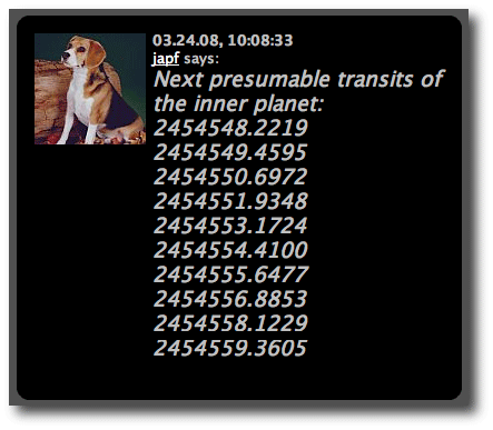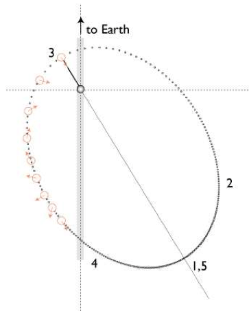
first quarter numbers

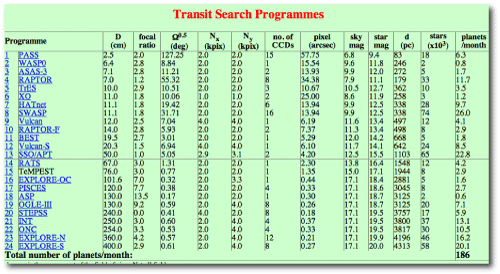
Back in 2002, Keith Horne gave a talk at the Frontiers in Research on Extrasolar Planets meeting at the Carnegie Institute in Washington and showed an interesting table:

At that time, there were more than two dozen active searches for transiting extrasolar planets, but only a single transiting planet — HD 209458 b — had been detected. Transits were generating a lot of excitement, but paradoxically, the community was well into its third straight year with no transit detections. The photometric surveys seemed to be just on the verge of really opening the floodgates, with a total theoretical capacity to discover ~200 planets per month.
It’s been six years, and the total transiting planet count is nowhere near 14,000. Most of the surveys on the table have had a tougher-than-expected time with detections because of the large number of false positives, and because of the need to obtain high-precision radial velocities on large telescopes to confirm candidate transiting planets. Indeed, the surveys that were sensitive to dimmer stars have largely faded out. It’s just too expensive to get high-precision velocities for V>15 stars. With the exception of the OGLE survey (which had been set up to look for microlensing during the 1990s, and which had established a robust pipeline early on) none of the surveys that employed telescopes with apertures larger than 12 cm have been successful. The currently productive photometric projects: TrES, XO, HATnet, and SuperWASP all rely on telescopes of 10 to 11 cm aperture to monitor tens of thousands to hundreds of thousands of stars, and all are sensitive to planets transiting stars in the V~10 to V~12 magnitude range. This magnitude range is the sweet spot: there are plenty of stars (and hence plenty of transits) and the stars are bright enough for reasonably efficient radial velocity confirmation.
Yesterday, SuperWASP rolled out 10 new transits at once, dramatic evidence of the trend toward planetary commoditization and of the fact that it’s getting tougher to make a living out on the discovery side. The detection of new planets is growing routine enough that in order to generate a news splash, you need multiple planets, and the more the better. This inflationary situation for new transit news is highly reminiscent of where the Doppler surveys were at seven years ago. For example, on April 4, 2001, the Geneva team put out a press release announcing the discovery of eleven new planets (including current oklo fave HD 80606b).

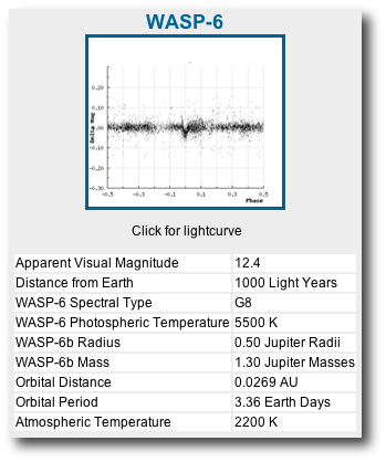
I’d like to register some annoyance with this latest SuperWASP announcement. There are no coordinates for the new planets, making it impossible to confirm the transits. There is no refereed paper. The data on the website are inconsistent, making it hard to know what’s actually getting announced. I was astonished, for example, that WASP-6 is reported on the website to have a radius 50% that of Jupiter, and a mass of 1.3 Jovian masses:

That’s nuts! If the planet is so small, why is the transit so deep? And a 2200 K surface temperature for a 3.36d planet orbiting a G8 dwarf? Strange. Perhaps the radius and mass have been reversed? In addition, there are weird inconsistencies between the numbers quoted in the media diagram and in the tables. For example, the diagram pegs WASP-7 at 0.67 Jovian masses, whereas the table lists it at 0.86 Jovian masses. WASP-10 has a period of 5.44 days in the table and 3.093 days in the summary diagram. Putting out a press release without the support a refereed paper is never a very good idea, even when there’s a danger that another team will steal your thunder with an even larger batch of planets.

Despite the difficulty in getting accurate quotes from the exchange, it’s interesting to see how the ten new planets stack up in the transit pricing formula. Using the data from the new WASP diagram (except for the 0.66 day period listed for WASP-9) and retaining the assumption that USD 25M has been spent in aggregate on ground-based transit searches, the 46 reported transits come out with the following valuations:

Planet Value
CoRoT-Exo-1 b $78,818
CoRoT-Exo-2 b $48,558
Gliese 436 b $3,970,811
HAT-P-1 b $883,671
HAT-P-2 b $77,938
HAT-P-3 b $260,473
HAT-P-4 b $172,851
HAT-P-5 b $133,239
HAT-P-6 b $224,110
HAT-P-7 b $54,382
HD 149026 b $722,590
HD 17156 b $869,254
HD 189733 b $2,429,452
HD 209458 b $10,103,530
Lupus TR 3 b $17,488
OGLE TR 10 b $60,260
OGLE TR 111 b $74,524
OGLE TR 113 b $36,599
OGLE TR 132 b $12,326
OGLE TR 182 b $15,261
OGLE TR 211 b $18,653
OGLE TR 56 b $19,761
SWEEPS 04 $1,826
SWEEPS 11 $193
TrES-1 $556,308
TrES-2 $113,043
TrES-3 $93,018
TrES-4 $205,508
WASP-1 $190,539
WASP-2 $188,956
WASP-3 $105,284
WASP-4 $104,581
WASP-5 $65,926
WASP-6 $339,387
WASP-7 $402,125
WASP-8 $209,169
WASP-9 $106,532
WASP-10 $74,281
WASP-11 $233,334
WASP-12 $160,189
WASP-13 $461,104
WASP-14 $14,450
WASP-15 $243,780
XO-1 $436,533
XO-2 $375,996
XO-3 $33,367

The ten new WASP planets (assuming that the correct parameters have been used) contribute about 1/10th of the total catalog value. There will likely be interesting follow-up opportunities on these worlds from ground and from space, but its unlikely that they’ll rewrite the book on our overall understanding of the field.

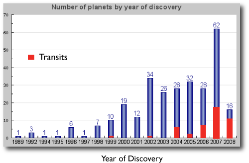
It’s interesting to plot the detection rate via transits in comparison to the overall detection rate of extrasolar planets. (The data for the next plot was obtained using the histogram generators at the Extrasolar Planets Encyclopaedia, which are very useful and are always up-to-date.)

It’s a reasonable guess that 2008 will be the first year in which the majority of discoveries arrive via the transit channel, especially if CoRoT comes through with a big crop. Radial velocity, however holds an edge in that it’s surveying the brightest stars, and (so far) has been responsible for progress toward the terrestrial-mass regime. I think that we might be seeing planets of only a few Earth masses coming out of the RV surveys during the coming year. Certainly, everything else being equal, a planet orbiting an 8th magnitude star is far more useful for follow-up characterization than a planet orbiting a 13th magnitude star.

1:1 eccentric

Image Source.

The range of planetary orbits that are observed in the wild is quite a bit more varied than the staid e < 0.20 near-ellipses in our own solar system. For regular oklo readers, the mere mention of Gl 876, 55 Cancri, or HD 80606, is enough to bring to mind exotic worlds on exotic orbits.

Non-conventional configurations involving trojan planets have been getting some attention recently from the cognescenti. Even hipper, however, is a configuration that I’ll call the 1:1 eccentric resonance. Two planets initially have orbits with the same semi-major axis, but with very different eccentricities. Conjunctions initially occur close to the moment of apoastron and periastron for the eccentric member of the pair.

Here’s a movie (624 kB Mpeg) of two Jupiter-mass planets participating in this dynamical configuration.

At first glance, the system doesn’t look like it’ll last very long. Remarkably, however, it’s completely stable. Over the course of a 400-year cycle, the two planets trade their angular momentum deficit back and forth like a hot potato and manage to orbit endlessly without anyone getting hurt.

Here’s an animation (1 MB Mpeg) which shows a full secular cycle. The red and the blue dots show the planet positions during the two orbit crossings per orbit made by one of the planets. It’s utterly bizarre.

These animations were made several years ago by UCSC grad student Greg Novak (who’ll be getting his PhD this coming summer with a thesis on numerical simulations of galaxy formation and evolution). As soon as we can get the time, Greg and I are planning to finish up a long-dormant paper that explores the 1:1 eccentric resonance in detail. In short, these configurations might be more than just a curiosity. When planetary systems having three or more planets go unstable, two of the survivors can sometimes find themselves caught in the 1:1 eccentric resonance. The radial velocity signature of the resulting configuration is eminently detectable if the planets can be observed over a significant number of orbital periods.

one seven one five six redux

Image Source.

Stefano, and Eugenio and I have been completely immersed in several time-critical projects during the past few months, and as a result, the frequency of posts here on oklo.org has not been as high as I would like. We’re starting to see our way clear, however, and very shortly, there’ll be a number of significant developments to report. Also in the cards is a major new release of the console, and a refocus on the research being carried out on the systemic backend. In any case, sincere thanks to all the backend participants for their patience.

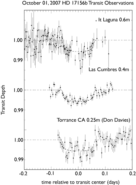
Oklo regulars will recall all the excitement last fall surrounding the discovery of transits by HD 17156b. The transit was first observed on September 10th by a cadre of small telescope observers, and was then confirmed 21.21 days later on October 1.

Jonathan Irwin at Harvard CfA has led the effort to analyze and publish the October 1 observations of the transit. The work recently cleared the peer-review process, and was posted on the web a few days ago. (Here’s a link to the paper on astro-ph.)

The night of October 1 was plagued by atrociously aphotometric conditions across the North American continent, and most of the observers who tried to catch the transit were clouded out. Southern California, however, had reasonably clear skies, and three confirming time series came from the Golden State. The Mount Laguna observations were taken from SDSU’s Observatory in the mountains east of San Diego, the Las Cumbres observations were made from the parking lot of the LCOGT headquarters in Santa Barbara, and Transitsearch.org participant Don Davis got his photometry from his backyard in suburban Los Angeles.

The aggregate of data from the October 1 transit allowed us to refine the orbital properties of the planet, and additional confirming observations in a paper by Gillon (of ‘436 fame) et al have given a much better characterization of the orbit.

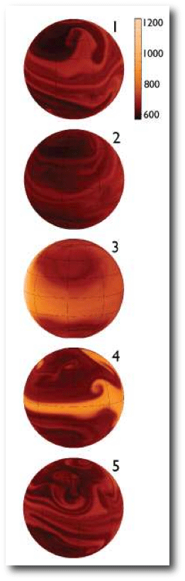
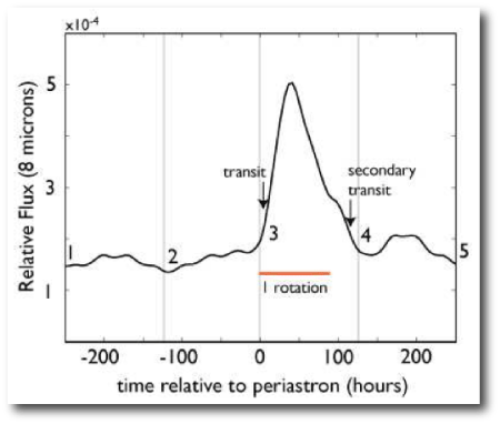
Because of the high orbital eccentricity, the planet should have very interesting weather dynamics on its surface. Jonathan Langton’s model predicts that the planet’s 8-micron flux should peak strongly during the day or so following periastron passage as the heated hemisphere of the planet turns toward Earth.

By measuring the rise and subsequent decay of the planet’s infrared emission, it’ll be possible to get both a measure of the effective radiative time constant in the atmosphere as well as direct information regarding the planet’s rotation rate. Bryce Croll is leading a team that successfully obtained time on the Spitzer telescope to make the observations.

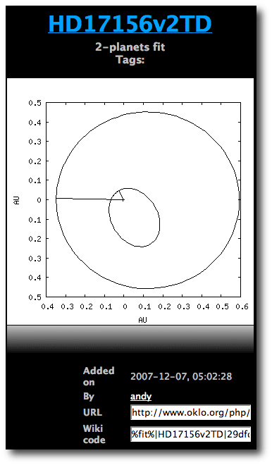
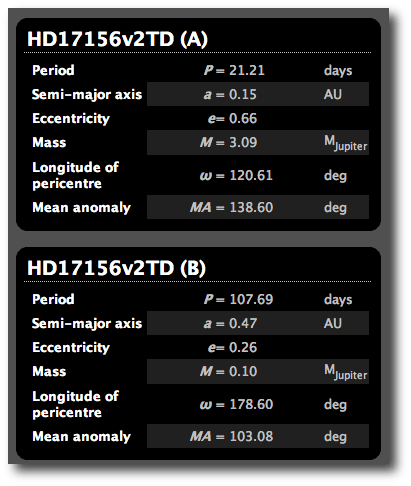
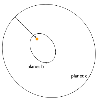
In another interesting development, a paper by Short et al. appeared on astro-ph last week which proposes the existence of a second planet in the HD 17156 system. The Short et al. planet has an Msin(i) of 0.06 Jupiter masses and an orbital period of 111.3 days. It’s quite similar to the slightly more eccentric (and hence dynamically unstable) version of the HD 17156 system proposed by Andy on the Systemic Backend last December, which was based on the radial velocities and transit timing then available:


The existence of a second planet in the HD 17156 system would be extremely interesting! The immediate question, however, is, how likely is it that the second planet is actually there?

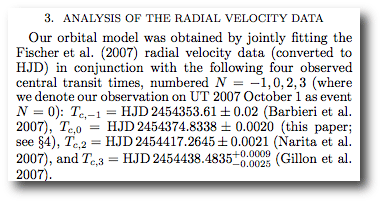
To make an independent investigation, it’s straightforward to use the downloadable systemic console to fit to the available published data on HD 17156. I encourage you to fire up a console and follow along. Now that the Irwin et al. paper is on the web, we have the following transit ephemerides:

These can be added to the HD17156.tds transit timing file in the datafiles directory. The file should be edited to look like this:

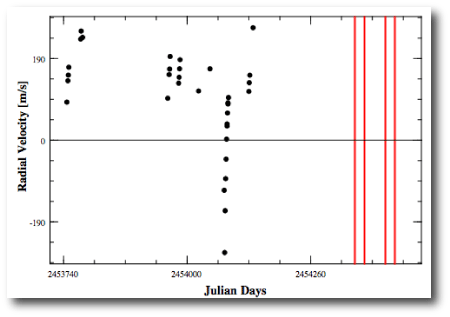
When the HD17156v2TD system is opened on the console, it shows both the radial velocity and the transit timing data.

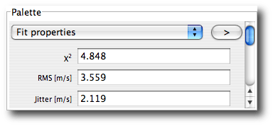
It’s quick work to dial in a one planet fit to the RV and transit timing data. I get a system with the following fit statistics:

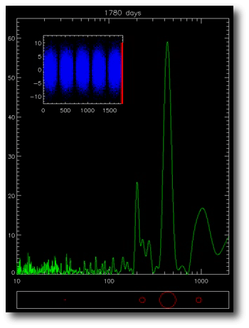
The required jitter of 2.12 m/s indicates that a one planet fit to the data should still be perfectly adequate, since the star (which is fairly hot and massive) has an expected stellar jitter of order 3 m/s. Nevertheless, the residuals periodogram does show a distinct peak at ~110 days:

Using the 110 day frequency as a starting point, one finds that ~0.1 Mjup planets do indeed lower the chi-square. I’ve uploaded an example two planet fit to the systemic backend that harbors a second planet in a 113 day orbit and a mass of 0.13 Jupiter masses. Its periastron is aligned with that of planet b, and the RMS has dropped down to 3.08 m/s (for a self-consistent, integrated fit). The implied stellar jitter is a bargain-basement 0.59 m/s, which is almost certainly too good to be true.

When I do an F-test between my one and two planet fits, the false alarm probability for planet ccomes in at 38%. It’s thus fairly likely that the second planet is spurious, but nevertheless, it certainly could be there, and it’ll be very interesting to keep tabs on both the transit timing data and the future radial velocity observations of this very interesting system…

Hawaii

Image Source.

Over the past two days, I got the opportunity to fly to Hawaii to give two talks for the Keck Observatory’s Evening With Astronomers series. The talks focused on extrasolar planets (here’s a link to the slides in Quicktime format, ~40MB , along with the audio files of (1) a planetary system in a 2:1 resonance, (2) an unstable planetary system, and (3) another unstable system). Both talks were on Kona coast of the Big Island, where, behind the palm trees, Mauna Kea looms up 13,796 feet in the hazy volcanic distance.

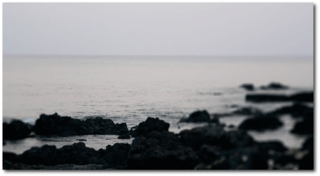
The landscape here resembles nothing so much as a habitable, terraformed Mars. Hardened ropes of lava run down to the water’s edge:

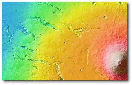
In the pre-dawn light this morning, the air was totally silent, and it was easy to imagine that I was actually on Mars, before the water was gone, when a Northern hemispheric ocean lapped up against the lava of the lowermost slopes of Elysium Mons:

Image Source.

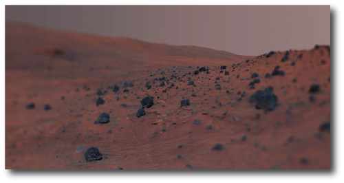
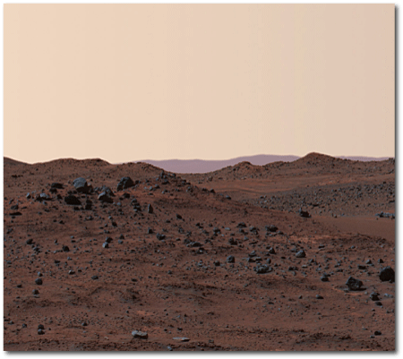
In the last few years the Martian landscape has become much more familiar, as the Spirit and Opportunity rovers crawl across the surface and radio home their photographs:

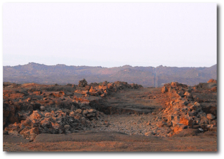
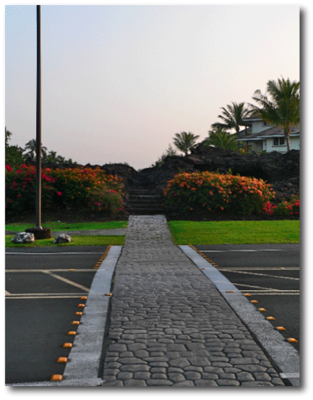
At Kona, looking out toward the lava fields, the view is positively Martian, with the most immediate difference being a sky that is a hazy blue-white rather than a hazy salmon-white. Here, the Ala Loa trail recedes into the jagged distance of what could easily be Mars:

On Mars, however, one generally has a fairly reasonable sense of what the 360-degree panorama will look like even if only part of the horizon is in view. On Earth, the situation can be quite different. Here’s the view that one gets simply by turning and looking in the opposite direction down the Ala Loa trail:

(On a marginally related note, our Alpha Centauri ApJ paper is starting to pick up some news coverage. Here’s a link to a story by National Geographic News.)

And four point five billion years later…

Image Source.

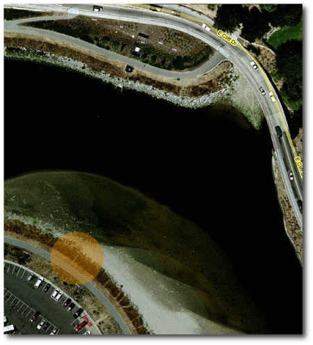
The last mile of the San Lorenzo river in Santa Cruz is strongly affected by the twice-daily ebb and flow of the tides.

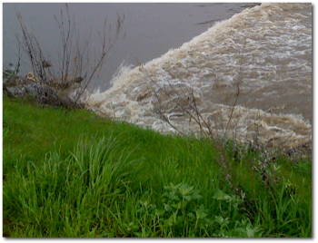
It’s always startling to see the tidal bore, a solitary breaking wave that runs upstream at a ~8 minute per mile pace when the tide is coming in. The San Lorenzo bore is small, usually six to nine inches high, but dramatic nonetheless. In its wake, there’s a turbulent froth of whitewater, whose eddies eventually cascade into viscous dissipation, turning the kinetic energy of organized flow into a slight heating of the water. As the Moon recedes, the Earth spins down, and the bore expends itself in a swirl of eddies.

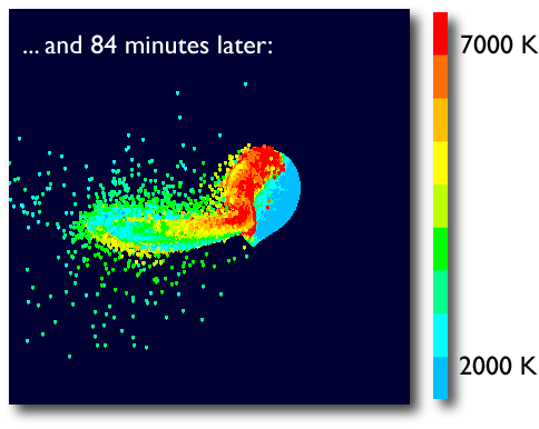
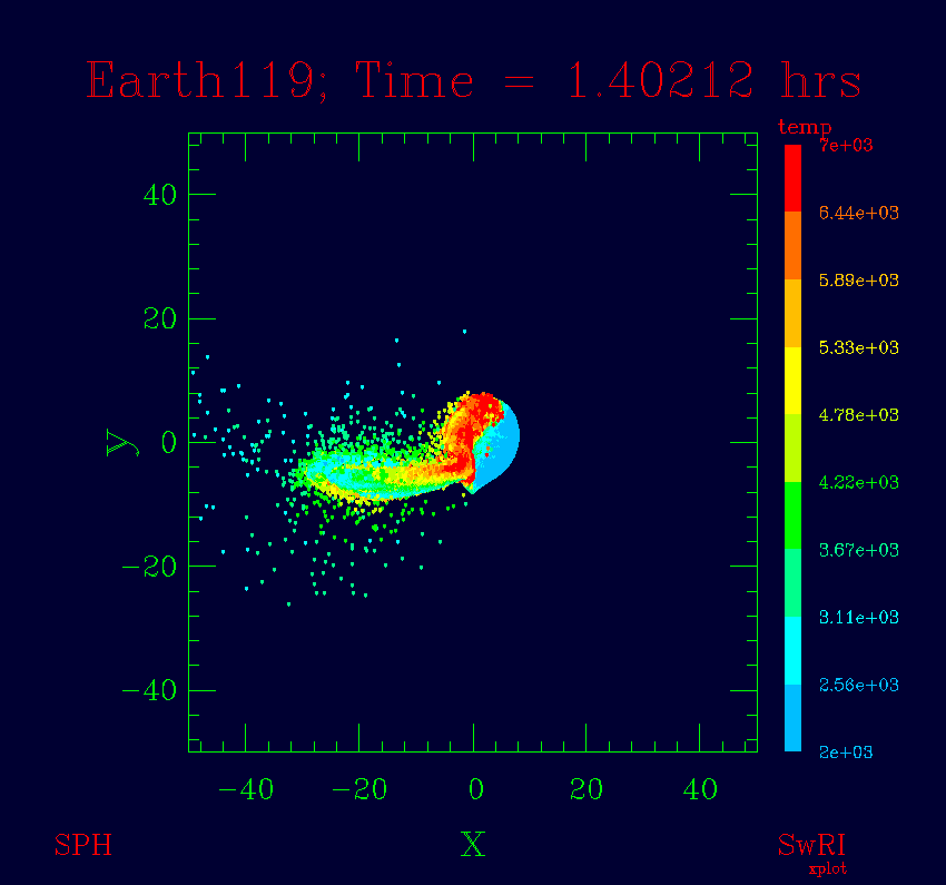
The energy that powers the bore was all imparted during the Moon-forming impact, in which a Mars-sized object collided with Earth, leaving the planet violently shaken and stirred and spinning crazily through days that were originally just a few hours long. Now, 4.5 billion years later, the bore running up the river is a distant echo of the impact that was large enough to cause Earth to glow with the temperature of a red dwarf star.

From Robin Canup's moon-forming impact simulation

Adapted from: Source.

There’s a nice discussion of tidal bores in the 1899 popular-level book The Tides and Kindred Phenomena in the Solar System, by Sir G. H. Darwin (son of the naturalist). The book in its entirety can be downloaded from The Internet Archive.

The Moon-forming impact, which occurred somewhere between 10 and 100 million years after the collapse of the pre-solar molecular cloud core, essentially marked the end of terrestrial planet formation in our own solar system. From a dynamical standpoint, a system undergoes a lot of evolution during a time scale of 100 million orbits. By contrast, the Milky Way galaxy is only about 40 orbits old, and is still in an effectively pristine, dynamically unrelaxed configuration.

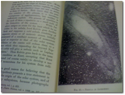
At Darwin’s time, the first photographs of spiral galaxies were appearing, and there’s a remarkably good photo of the Andromedae galaxy on page 339 of the book:

Darwin writes:

There is good reason for believing that the Nebular Hypothesis presents a true statement in outline of the origin of the solar system, and of the planetary subsystems, because photographs of nebulae have been taken recently in which we can almost see the process in action. Figure 40 is a reproduction of a remarkable photograph by Dr. Isaac Roberts of the great nebula in the constellation of Andromeda. In it we may see the lenticular nebula with its central condensation, the annulation of the outer portions, and even the condensations in the rings which will doubtless at some time form planets. This system is built on a colossal scale, compared with which our solar system is utterly insignificant. Other nebulae show the same thing, and although they are less striking we derive from them good grounds for accepting this theory of evolution as substantially true.

In 1899, the extragalactic distance scale hadn’t been established, and so Darwin thought that M31 was a lot closer than it actually is. In dynamical terms, he would have guessed that it’s many thousands of orbits old rather than only a few dozen. Nevertheless, it’s interesting to think about what will happen to an isolated spiral galaxy by the time it’s 10^18 years old…

Toward Alpha Cen B b

Image Source.

Yesterday, I gave a talk at the JPL Exoplanet Science and Technology Fair, a one-day meeting that showcased the remarkably broad variety of extrasolar planet-related research being carried out at JPL. In keeping with the wide array of projects, the agenda was fast-paced and completely diverse, with talks on theory, observation, instrumentation, and mission planning.

The moment I walked into the auditorium, I was struck by the out-there title on one of the posters: The Ultimate Project: 500 Years Until Phase E, from Sven Grenander and Steve Kilston. Their poster (pdf version here) gives a thumbnail sketch of how a bona-fide journey to a nearby habitable planet might be accomplished. The audacious basic stats include: 1 million travelers, 100 million ton vessel, USD 50 trillion, and a launch date of 2500 CE.

Fifty trillion dollars, which is roughly equivalent to one year of the World GDP, seems surprisingly, perhaps even alarmingly cheap. The Ultimate Project has a website, and for always-current perspective on interstellar travel, it pays to read Paul Gilster’s Centauri Dreams weblog.

Interest in interstellar travel would ramp up if a truly Earth-like world were discovered around one of the Sun’s nearest stellar neighbors. Alpha Centauri, 4.36 light years distant, has the unique allure. Last year, I wrote a series of posts [1, 2, 3, 4] that explored the possibility that a habitable world might be orbiting Alpha Centauri B. In short, the current best-guess theory for planet formation predicts that there should be terrestrial planets orbiting both stars in the Alpha Cen binary. In the absence of non-gaussian stellar radial velocity noise sources, these planets would be straightforward to detect with a dedicated telescope capable of 3 m/s velocity precision.

Over the past year, we’ve done a detailed study that fleshes out the ideas in those original oklo posts. The work was led by UCSC graduate student Javiera Guedes and includes Eugenio, Erica Davis, myself, Elisa Quintana and Debra Fischer as co-authors. We’ve just had a paper accepted by the Astrophysical Journal that describes the research. Javiera will be posting the article to astro-ph in the next day or so, but in the meantime, here is a .pdf version.

Here’s a diagram that shows the sorts of planetary systems one should expect around Alpha Cen B. The higher metallicity of the star in comparison to the Sun leads to terrestrial planets that are somewhat more massive.

We’re envisioning an all-out Doppler RV campaign on the Alpha Cen System. If the stars present gaussian noise, then with 3 m/s, one can expect a very strong detection after collecting data for five years:

Here’s a link to an animation on Javiera’s project website which shows how a habitable planet can literally jump out of the periodogram.

I think the planets are there. The main question in my opinion is whether the stellar noise spectrum is sufficiently Gaussian. It’s worth a try to have a look…

two for one deals?

Image Source.

The Gliese 876 system is remarkable for a number of reasons. It makes a mockery of the notion that the minimum-mass solar nebula has a universal validity. It harbors one of the lowest-mass extrasolar planets known (discovered by our own Eugenio Rivera). And of course, the outer two planets are famously caught in a 2:1 mean motion resonance, in which the inner 0.8 Jupiter-mass planet makes (on average) exactly two trips around the red dwarf for every one trip made by the outer 2.5 Jupiter-mass planet.

As users of the console know, the planet-planet interactions between the Gliese 876 planets are strong enough so that one needs a self-consistent dynamical fit to the system. Even on the timescale of a single outer planet orbit, the failure of the Keplerian model can be seen on a 450-pixel wide .gif image:

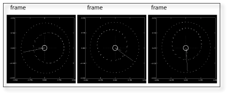
The following three frames are from a time-lapse .mpg animation of the Gliese 876 system over a period of roughly one hundred years:


Each frame strobes the orbital motion of the planets at 50 equally spaced intervals which subdivide the P~60 day period of the outer planet. Upon watching the movie, it’s clear that the apsidal lines of the outer two planets are swinging back and forth like a pendulum. This oscillation has an amplitude (or libration width) of 29 degrees, and acts like a fingerprint identifier of the Gliese 876 system.

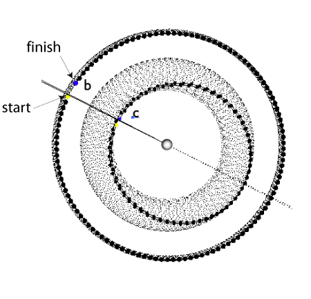
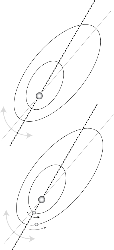
The derangement of the orbits is reflected in their continual inability to maintain an exact 2:1 orbital commensurability. The first figure up above shows that when planet c has finished exactly two orbits, it has already managed to lap planet b, which was still dawdling down Boardwalk prior to passing GO.

Planet b, however, doesn’t always run slow. The gravitational perturbations between the two planets provide a second pendulum-like restoring action which prevents the bodies from straying from the average period ratio of 2:1, which, over the long term, is maintained exactly. The degree to which the orbits themselves librate, combined with the planets’ abilities to run either ahead or behind exact commensurability is captured by the resonant arguments of the configuration. These can be defined as,

where the lambdas are mean longitudes and the curly pi’s are the longitudes of periastron. The two resonant arguments capture the simultaneous libration of the mean motions and the apsidal lines. The smaller the arguments, the more tightly the system is in resonance.

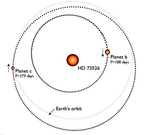
In the Gliese 876 system, the resonant arguments are both librating with amplitudes of less than 30 degrees. This is evidence that a dissipative mechanism was at work during the formation of the system. Interestingly, however, when one looks at the other extrasolar planetary systems that are thought to be in 2:1 resonance, one finds that the libration amplitudes in every case are much larger. In fact, in the HD 73526 system and in the HD 128311 system, only one of the arguments is librating, while the other is circulating. In this state of affairs, the apsidal lines act like a pendulum that is swinging over the top. In addition, the orbital eccentricites are higher, and the sum of planet-planet activity is strikingly greater (see this animation of the evolution of the HD 128311 system).

A gas disk seems to be the most likely mechanism for pushing a planetary system into mean-motion resonance. Protoplanetary disks are likely, however to experience turbulent density fluctuations. These density fluctuations lead to stochastic gravitational torques, which provide a steady source of orbital perturbations to any planets that are embedded in a disk. For a reasonable spectrum of turbulent fluctuations, it turns out that it’s rather difficult to wind up with a planetary system that is as deeply in resonance as Gliese 876. The conclusion, then, is that Gliese 876-like configurations should be quite rare. Indeed, 2:1 resonances of every stripe should constitute only a minor fraction of planetary systems, and the majority that do exist should either large libration widths or only a single argument in resonance.

If you’re interested in more detail, we’ve submitted a paper that goes into much more detail (Adams, Laughlin & Bloch, ApJ, 2008 Submitted).

436 again

Image Source.

There’s a provocative paper up on the astro-ph today. Ignasi Ribas and two collaborators are reporting the “possible discovery” of a 4.8 Earth mass planet in an exterior 2:1 mean motion resonance with the transiting hot Neptune Gliese 436b. Planet four three six b is the well-known subject of great consternation, great scientific value, and many an oklo.org post. (For the chronological storyline, see: 1 (for background), 2, 3, 4, 5, 6, 7, 8, 9, and 10.)

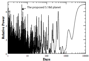
Here’s the basic idea. Ribas et al. note that a single-planet fit to the Maness et al. (2007) radial velocity data set (which is listed as gj_436_M07K on the systemic console) has a peak in the residuals periodogram at P~5.1866 days:

Using this periodogram peak as a starting point, they get a keplerian 2-planet fit that lowers the reduced chi-square from ~4.7 to ~3.7. They then point out that this detection can potentially be confirmed by measuring variations in transit timing. In their picture, the presently-grazing transit has come into visibility only within the last 2.5 years or so, as a result of orbital precession. The transit light curve should thus be showing significant variations in duration as well as deviations from a strictly periodic sequence of central transit times.

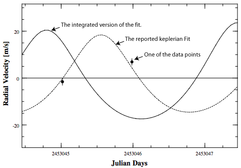
This will be a huge big deal if the claim holds up. For starters, it’ll provide a natural explanation for Gl 436b’s outsize eccentricity. And everyone’s been on the lookout for a strongly resonant transiting system with a short orbital period. For the time being, though, I’m withholding judgment. As a first point of concern, Ribas et al. are presenting a keplerian fit to the radial velocities. Yet for the orbital configuration they are proposing, it’s absolutely vital to take planet-planet interactions into account. One can see this by entering their fit into the console. (Use a mean anomaly at the first RV epoch 2451552.077 for planet b=40.441 deg, corresponding to their reported time of periastron of Tp_b=HJD 2451551.78, and a mean anomaly for planet c=268.14 deg, corresponding to their reported value of Tp_c=HJD 2451553.4.) One can also dial in a long-term trend if one wants, but this isn’t necessary. Once the fit is entered, the reduced chi-square is 3.7. Activate integration. (Hermite 4th-order is the faster method.) When the planets are integrated, their mutual interactions utterly devastate the fit, driving the reduced chi-square up to 85.018. Using the zoomer and the scroller, you’ll see that the integrated radial velocity curve and the keplerian curve start off as a good match, but then rapidly get completely out of phase.

In order to examine the plausibility of a two-planet fit in 2:1 mean motion resonance, one needs to fit the radial velocity data with integration turned on. It is also important to include the existing transit timing data in the fit (and to do this, it’s best to use the most recent, so-called unstable version of the console). Over at Bruce Gary’s amateur exoplanet archive (AXA), there are now three transit timing measurements listed, with the latest obtained by Bruce himself this past New Years Eve. The HJD measurements of central transit should be added to the gj436.tds file, along with the HJD 2454280.78149 +/- 0.00016 central transit time measured by Spitzer.

Ideally, the Spitzer secondary transit timing data should also be included, but at the moment, the distribution version of the console does not have the capability to incorporate secondary transit measurements. One approach would be to get a self-consistent fit, and then see whether the epoch of secondary transit matches that observed by Spitzer.

Have fun…

Messenger

Image Source.

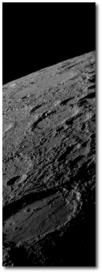
Messenger flew by Mercury last week, and photographed vast swaths of terrain that, until now, had never been seen. The new landscapes, as expected, are cratered, barren, and utterly moonlike. The galaxy could contain a hundred billion planets that would be hard, at first glance, to distinguish from Mercury, and within our cosmic horizon, there are probably of order as many Mercury-like worlds as there are sucrose molecules in a cube of sugar.

Image Source.

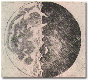
Nevertheless, we do gain something extraordinary whenever a new vista onto a terrestrial world is opened up. Galileo was the first to achieve this, when he turned his telescope to the Moon and saw its three-dimensional relief for the first time. Mariner 4 and Mariner 9 accomplished a similar feat for Mars. The Magellan spacecraft revealed the Venusian topography. And once Messenger has photographed the full surface of Mercury, there will be a profoundly significant interval before we get our next up-close view of an unmapped terrestrial planet. My guess is that it’ll be Alpha Centauri B b.

The Messenger website is well worth a visit. I was particularly struck by the movie that the spacecraft made of the Earth during the close fly by of March 2005. During the course of 24 hours, the spinning Earth recedes into the black velvet distance and space travel seems like the real thing.

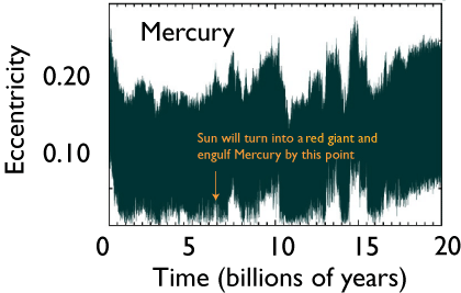
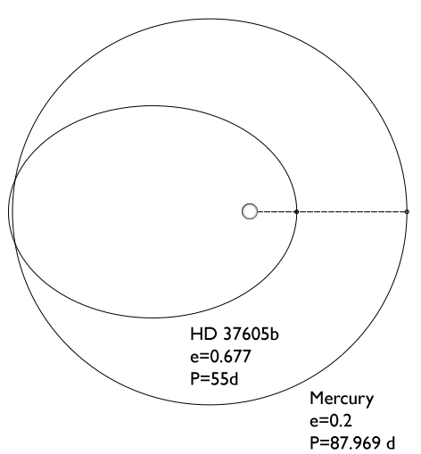
Mercury’s orbit, with its 88 day period and its eccentricity of 0.2 could slip unnoticed into the distribution of known exoplanets. It’s vaguely comparable, for example, with the orbit of HD 37605 b. This Msini=2.3 Mjup gas giant has an apoastron distance similar to Mercury’s, but dives much closer to its star during periastron.

We’ve been interested in HD 37605 b lately because its orbit dips in and out of the insolation zone where water clouds are expected to exist. At the far point of the 55 day orbit, it should be possible for white clouds to form out of a clear steamy atmosphere. At close approach, the clouds are turning to steam.

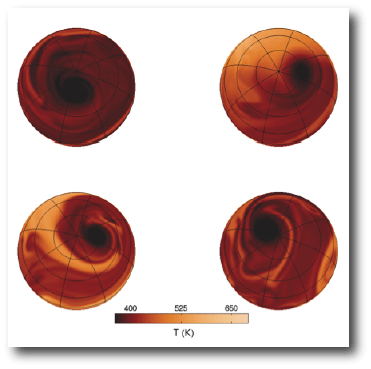
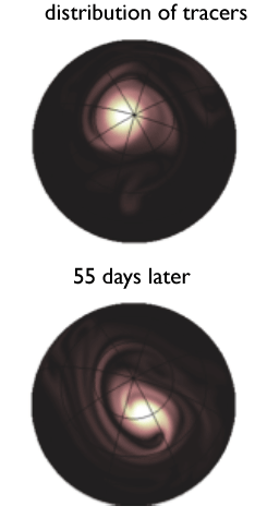
Jonathan Langton’s models for this planet show persistent polar vortices, which sequester cooler air, and which may remain cloudy even during the hot days surrounding periastron. The vortices are tenaciously long-lived, and tracer particles seeded into the vortices leak out only slowly. It would be interesting to know what sort of chemistry is brewing in the steamy hothouse environment of trapped and noxious air.

Sir, I have no need of that hypothesis!

Image Source.

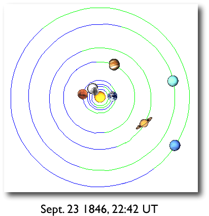
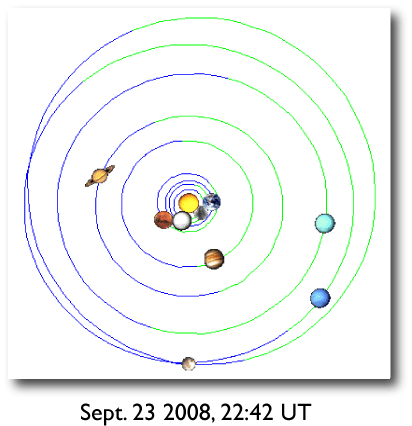
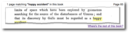
On the UCSC Science Library shelves, we have an 1828 edition of Pierre Simon de Laplace’s Oeuvres that includes the five-volume Mecanique Celeste. At moments like this, it’s great to have a camera on one’s cellphone:

Image Source.

Laplace’s identification of the 5:2 near-resonance between Jupiter and Saturn allowed him to augment the exisiting second-order Laplace-Lagrange secular analysis to produce a theory of planetary motion that was in extraordinary agreement with the observations of the late eighteenth century. His success in explaining the so-called Great Inequality was likely a contributing factor in the development the concept of Laplacian determinism, of a clockwork universe.

In 1802, during William Herschel’s visit to Paris, Herschel and Laplace had a meeting with Napoleon, who, like Thomas Jefferson, appears to have been not much taken with a system of the world created and dictated by natural law:

The first Consul then asked a few questions relating to Astronomy and the construction of the heavens to which I made such answers as seemed to give him great satisfaction. He also addressed himself to Mr. Laplace on the same subject, and held a considerable argument with him in which he differed from that eminent mathematician. The difference was occasioned by an exclamation of the first Consul, who asked in a tone of exclamation or admiration (when we were speaking of the extent of the sidereal heavens): “And who is the author of all this!” Monsieur De la Place wished to shew that a chain of natural causes would account for the construction and preservation of the wonderful system. This the first Consul rather opposed.

[Source: Herschel’s diary of his visit to Paris in 1802, as found in C. Lubbock’s _The Herschel Chronicle_, p. 310, see here for a nice background.]

I like the extrasolar planet game because it’s simultaneously up-to-the-minute and steeped in tradition. With systems like Gliese 876, we’re approaching roughly the same effective degree of refinement in our detection of planet-planet orbital perturbations that was possible in the late eighteenth century for Jupiter and Saturn. As a result, someone like Laplace, were he to materialize (see today’s NYT) in the Interdisciplinary Sciences Building here at UCSC, could roll up his french cuffs and immediately begin contributing publishable work. The same would certainly not be true if one of his equally luminous scientific contemporaries, say Antoine Lavoisier, were to suddenly walk in to a modern-day chemistry lab.

Will be making an effort to post more frequently. Thanks for your continued readership and participation as oklo.org heads into its third year.

transit valuations

Image Source

Discoveries relating to transiting extrasolar planets often make the news. This is in keeping both with the wide public interest in extrasolar planets, as well as the effectiveness of the media-relations arms of the agencies, organizations, and universities that facilitate research on planets. I therefore think that funding support for research into extrasolar planets in general, and transiting planets in particular, is likely to be maintained, even in the face of budget cuts in other areas of astronomy and physics. There’s an article in Saturday’s New York Times which talks about impending layoffs at Fermilab, where the yearly budget has just been cut from $342 million to $320 million. It’s often not easy to evaluate how much a particular scientific result is “worth” in terms of a dollar price tag paid by the public, and Sean Carroll over at Cosmic Variance has a good post on this topic.

For the past two years, the comments sections for my oklo.org posts have presented a rather staid, low-traffic forum of discussion. That suddenly changed with Thursday’s post. The discussion suddenly heated up, with some of the readers suggesting that the CoRoT press releases are hyped up in relation to the importance of their underlying scientific announcements.

How much, actually, do transit discoveries cost? Overall, of order a billion dollars has been committed to transit detection, with most of this money going to CoRoT and Kepler. If we ignore the two spacecraft and look at the planets found to date, then this sum drops to something like 25 million dollars. (Feel free to weigh in with your own estimate and your pricing logic if you think this is off base.)

The relative value of a transit depends on a number of factors. After some revisions and typos (see comment section for this post) I’m suggesting the following valuation formula for the cost, C, of a transit:

The terms here are slightly subjective, but I think that the overall multiplicative effect comes pretty close to the truth.

The normalization factor of 580 million out front allows the total value of transits discovered to date to sum to 25 million dollars. The exponential term gives weight to early discoveries. It’s a simple fact that were HD 209458 b discovered today, nobody would party like its 1999 — I’ve accounted for this with an e-folding time of 5 years in the valuation.

Bright transits are better. Each magnitude in V means a factor of 2.5x more photons. My initial inclination was to make transit value proportional to stellar flux (and I still think this is a reasonable metric). The effect on the dimmer stars, though was simply overwhelming. Of order 6 million dollars worth of HST time was spent to find the SWEEPS transits, and with transit value proportional to stellar flux, this assigned a value of two dollars to SWEEPS-11. That seems a little harsh. Also, noise goes as root N.

Longer period transits are much harder to detect, and hence more valuable. Pushing into the habitable zone also seems like the direction that people are interested in going, and so I’ve assigned value in proportion to the square root of the orbital period. (One could alternately drop the square root.)

Eccentricity is a good thing. Planets on eccentric orbits can’t be stuck in synchronous rotation, and so their atmospheric dynamics, and the opportunities they present for interesting follow-up studies make them worth more when they transit.

Less massive planets are certainly better. I’ve assigned value in inverse proportion to mass.

Finally, small stars are better. A small star means a larger transit depth for a planet of given size, which is undeniably valuable. I’ve assigned value in proportion to transit depth, and I’ve also added a term, Np^2, that accounts for the fact that a transiting planet in a multiple-planet system is much sought-after. Np is the number of known planets in the system. Here are the results:

Planet Value
CoRoT-Exo-1 b $86,472
CoRoT-Exo-2 b $53,274
Gliese 436 b $4,356,408
HAT-P-1 b $969,483
HAT-P-2 b $85,507
HAT-P-3 b $285,768
HAT-P-4 b $189,636
HAT-P-5 b $146,178
HAT-P-6 b $245,873
HD 149026 b $792,760
HD 17156 b $953,665
HD 189733 b $2,665,371
HD 209458 b $11,084,661
Lupus TR 3 b $19,186
OGLE TR 10 b $66,112
OGLE TR 111 b $81,761
OGLE TR 113 b $40,153
OGLE TR 132 b $13,523
OGLE TR 182 b $16,743
OGLE TR 211 b $20,465
OGLE TR 56 b $21,680
SWEEPS 04 $2,004
SWEEPS 11 $211
TrES-1 $610,330
TrES-2 $124,021
TrES-3 $102,051
TrES-4 $225,464
WASP-1 $209,041
WASP-2 $207,305
WASP-3 $115,508
WASP-4 $114,737
WASP-5 $72,328
XO-1 $478,924
XO-2 $506,778
XO-3 $36,607

HD 209458 b is the big winner, as well it should be. The discovery papers for this planet are scoring hundreds of citations per year. It essentially launched the whole field. The STIS lightcurve is an absolute classic. Also highly valued are Gliese 436b, and HD 189733b. No arguing with those calls.

Only two planets seem obviously mispriced. Surely, it can’t be true that HAT-P-1 b is 10 times more valuable than HAT-P-2b? I’d gladly pay $85,507 for HAT-P-2b, and I’d happily sell HAT-P-1b for $969,483 and invest the proceeds in the John Deere and Apple Computer corporations.

Jocularity aside, a possible conclusion is that you should detect your transits from the ground and do your follow up from space — at least until you get down to R<2 Earth radii. At that point, I think a different formula applies.

CoRoT-exo-2 c?

Image Source.

The CoRoT mission announced their second transiting planet today, and it’s a weird one. The new planet has a mass of 3.53 Jupiter masses, a fleeting 1.7429964 day orbit, and a colossal radius. It’s fully 1.43 times larger than Jupiter.

The surface temperature on this planet is likely well above 1500K. Our baseline theoretical models predict that the radius of the planet should be ~1.13 Jupiter radii, which is much smaller than observed. Interestingly, however, if one assumes that a bit more than 1% of the stellar flux is deposited deep in the atmosphere, then the models suggest that the planet could easily be swollen to its observed size.

The surest way to heat up a planet is via forcing from tidal interactions with other, as-yet unknown planets in the system. If that’s what’s going on with CoRoT-exo-2 b, then it’s possible that the perturber can be detected via transit timing. The downloadable systemic console is capable of fitting to transit timing variations in conjunction with the radial velocity data. All that’s needed is a long string of accurate central transit times.

The parent star for CoRoT-exo-2-b is relatively small (0.94 solar radii) which means that the transit is very deep, of order 2.3%. That means good signal to noise. At V=12.6, the star should be optimally suited for differential photometry by observers with small telescopes. With a fresh transit occurring every 41 and a half hours, data will build up quickly. As soon as the coordinates are announced, observers should start bagging transits of this star and submitting their results to Bruce Gary’s Amateur Exoplanet Archive. (See here for a tutorial on using the console to do transit timing analyses.)

6 Gigabytes. Two Stars. One Planet.

Image Source.

Another long gap between posts. I’m starting to dig out from under my stack, however, and there’ll soon be some very interesting items to report.

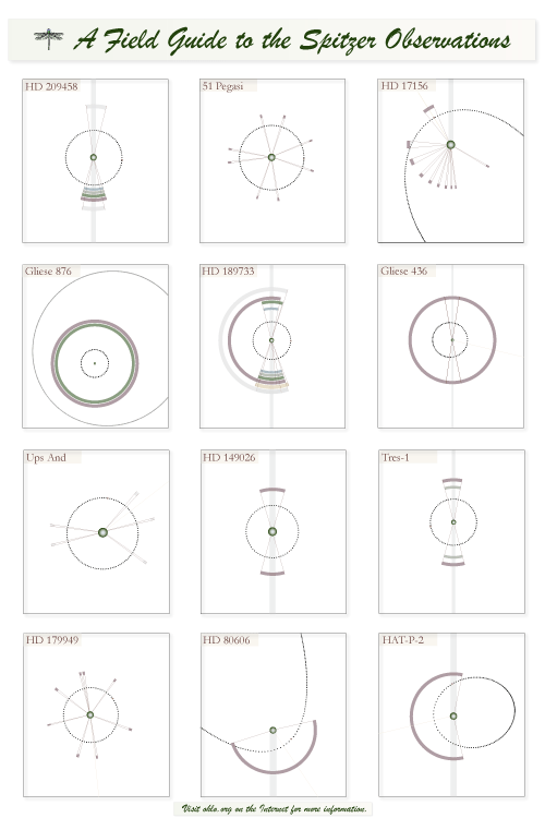
As mentioned briefly in the previous post, our Spitzer observations of HD 80606 did indeed occur as scheduled. Approximately 7,800 8-micron 256×256 px IRAC images of the field containing HD 80606 and its binary companion HD 80607 were obtained during the 30-hour interval surrounding the periastron passage. On Nov. 22nd, the data (totaling a staggering 6 GB) was down-linked to the waiting Earth-based radio telescopes of NASA’s Deep Space Network. By Dec 4th, the data had cleared the Spitzer Science Center’s internal pipeline.

We’re living in a remarkable age. When I was in high school, I specifically remember standing out the backyard in the winter, scrutinizing the relatively sparse fields of stars in Ursa Major with my new 20×80 binoculars, and wondering whether any of them had planets. Now, a quarter century on, it’s possible to write and electronically submit a planetary observation proposal on a laptop computer, and then, less than a year later, 6 GB of data from a planet orbiting one of the stars visible in my binoculars literally rains down from the sky.

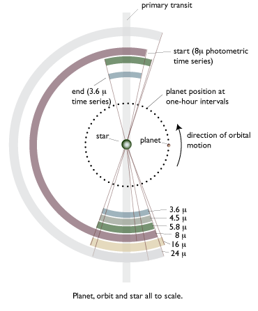
It will likely take a month or so before we’re finished with the analysis and the interpretation of the data. The IRAC instrument produces a gradually increasing sensitivity with time (known to the cognescenti as “the ramp”). This leads to a raw photometric light curve that slopes upward during the first hours of observation. For example, here’s the raw photometry from our Gliese 436 observations that Spitzer made last Summer. The ramp dominates the time series (although the secondary eclipse can also be seen):

The ramp differs in height, shape, and duration from case to case, but it is a well understood instrumental effect, and so its presence can be modeled out. Drake Deming is a world expert on this procedure, and so the data is in very capable hands. Once the ramp is gone, we’ll have a 2800-point 30 hour time series for both HD 80606 and HD 80607. We’ll be able to immediately see whether a secondary transit occurred (1 in 6.66 chance), and with more work, we’ll be able to measure how fast the atmosphere heats up during the periastron passage. Jonathan Langton is running a set of hydrodynamical simulations with different optical and infrared opacities, and we’ll be able to use these to get a full interpretation of the light curve.

In another exciting development, Joe Lazio, Paul Shankland, David Blank and collaborators were able to successfully observe HD 80606 using the VLA during the Nov. 19-20 periastron encounter! It’s not hard to imagine that there might be very interesting aurora-like effects that occur during the planet’s harrowing periastron passage. If so, the planet might have broadcasted significant power on the decameter band. Rest assured that when that when their analysis is ready, we’ll have all the details here at oklo.org.

planet per week

Image Source.

As the academic quarter draws to a close, it gets harder to keep up a regular posting schedule. This year, certainly, the difficulty has nothing to do with a lack of exciting developments associated with extrasolar planets.

A few unrelated items:

It appears that the HD 80606b Spitzer observations went smoothly, and that the data has been safely transmitted to Earth via NASA’s Deep Space Network. It is currently in the processing pipeline at the Spitzer Science Center. When it clears the pipeline, the analysis can start.

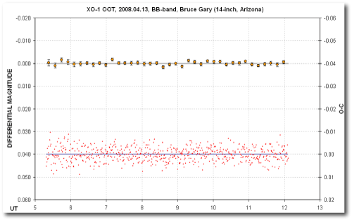
Back in September, I wrote a post about Bruce Gary’s Amateur Exoplanet Archive. This is a web-based repository for photometric transit observations by amateurs. With the number of known transits growing by the month, there’s a planet in transit nearly all of the time. Over 90 light curves have been submitted to the archive thus far. For transiting planets such as HD 189733b or HD 209458b, which have significant numbers of published radial velocity data, it’s very interesting to take the transit center measurements from Bruce’s archive and use them as additional orbital constraints within the console. The September post gives a tutorial on how to do this.

It really is turning out to be a banner year for extrasolar planets. As we head into December, this year is averaging more than one planet per week. The detection rate is more than double that of the previous four years.

The plot above gives a hint that Saturn-mass planets might wind up being fairly rare, as one might expect from the zeroth-order version of the core accretion theory. (For more information, this series: 1, 2, 3, 4, 5, 6, and 7 of oklo posts compares and contrasts the gravitational instability and core accretion theories for giant planet formation.)
Also, if you give talks, here’s a larger version of the above figure.

Another interesting diagram is obtained by plotting orbital period vs. year of discovery:

It’s possible that this diagram might be hinting that true Jupiter analogs are relatively rare. Could be that the disks around metal-rich stars are able to form Jovian mass planets and then migrate them in, while stars with subsolar metallicity form ice giants beyond the ice line. In this scenario, our solar system lies right on the boundary between the two outcomes.

It could also be the case that there are a whole slew of true-Jupiter analogs just on the verge of being announced. Time will tell.

And as always, it’s interesting to spend time with the correlation diagram tool over at exoplanet.eu.

160 basis points

Image Source.

It’s sometimes a little weird to realize that my daily schedule is dictated by the orbits of alien planets. HD 80606b went through periastron passage at 07:00 UT last Tuesday, with the Spitzer Space Telescope’s rattlesnake’s eye vision trained intently upon it. Over the past few days, it’s been hurtling away from the star, gradually reducing its velocity as it climbs up the gravitational potential well of the star.

At 07:45 UT on Monday morning, HD 80606b is scheduled to go through inferior conjunction. In the 1.6% a-priori geometric chance that the orbital plane of the planet is in near-perfect alignment with the line of sight to the solar system, then it will be possible to observe the planet in transit. The 1.6% transit probability is fairly high for a planet with a period of 111 days, but much lower than the 15% probability that a secondary eclipse can be observed. If the planet is undergoing secondary eclipse, then we’ll know as soon as the Spitzer data comes in.

Back in early 2005, Transitsearch.org coordinated a campaign to check for transits of HD 80606b. At that time, there were fewer radial velocities available, and so the transit window was less well constrained. A number of observers got data, and there was no sign of transit, but the coverage was not good enough to rule out a transit. I’m thus encouraging observers to monitor HD 80606 during the next 48 hours on the off chance that it can be observed in transit. Given the small chance involved, it seems appropriate to refer to the transit probability in terms of basis points. As in, “In ’05, we got about 40 basis points. That means there’s still 120 basis points out there to collect.”

HD 80606 is a visual binary. The companion, HD 80607, provides a good comparison star in telescopes with a large enough aperture under good seeing conditions. For most observers, however, the light from the two stars is combined. A transit by HD 80606b is expected to have a depth of order 1.4%, and (if it’s a central transit) will last about 16 hours. It’s a long-shot for sure, but worthwhile and fun nonetheless.