backlog

Image Source.

It was the end of the Winter quarter here at UCSC last week, and then I went on a trip, and then bam! More than a week with no posts… In the interim, there have been a number of interesting developments related to extrasolar planets. Here’s a brief run-down of some topics that I want to look at in more depth in the very near future:

Thanks to continuing efforts from the back-end user base, we’re accumulating a highly useful database of stable, low chi-square fits to the synthetic radial velocity data sets that comprise the Systemic Jr. catalog. Stefano has run a preliminary analysis and interpretation of the data. There are interesting implications for the overall eccentricity distribution of extrasolar planets, and there also appears to be a robust criterion for determining with confidence when you’ve extracted a real, previously unannounced planet from a given data set. We’re putting together a full report, which will appear quite soon. In the meantime, please keep submitting fits for systems that haven’t yet been adequately characterized.

The detection of another Neptune-mass planet orbiting a nearby red-dwarf was announced today. Yet more evidence for the core-accretion theory of planet formation! The discovery paper stops short of tabulating the radial velocities, but as I write this, Eugenio is busy dextering them onto the systemic back-end and onto the downloadable systemic console.

The theoretical case for the existence of Alpha Centauri B b is getting stronger by the day.

This year’s first ‘606 day is coming up next week, with a transit opportunity following on April 17th. I didn’t do enough to get the word out last December, but I’m hoping for good photometric coverage of the star during the upcoming window. A central transit for HD 80606b would last roughly 18 hours, so participation from observers worldwide will be required to definitively rule out transits.

Systemic Jr. Fit Drive

Image Source.

A big thank-you to everyone who’s been participating in the drive to characterize and study the catalog of synthetic “Systemic Jr.” planetary systems on the Systemic Backend. There’s now enough data to indicate that the analysis is going to be very informative. We’re looking forward to revealing the properties of the underlying planetary systems that were used to generate the data. In the meantime, we need your help to adequately characterize all 520 systems. Data in need of better characterization are marked by flags:

Our backend server is now swarming with various hard-working software robots that Stefano has assembled. The 100-year stability bot is rousted out of bed and set to work whenever a new fit is submitted. It reports a quick initial assessment of orbital stability. Planetary systems that pass through the 100-year stability screen are then put in a queue to wait for the attentions of the 1000-year stability bots. Systems that make it through 1000 years with less than a 1% change in semi-major axis of their planets are awarded a snazzy green flag:

Occasionally, systems that are in mean-motion resonance can show periodic semi-major axis variations of more than 1% while still remaining indefinitely stable. A resonance bot that will go through the fits and check for these special cases is currently being readied.

Systems that pass the minimum stability requirement are handed to a bootstrap bot which uses the bootstrap method to estimate uncertainties on the planetary orbital parameters for each stable fit. We’re currently running the bootstrap bot under the assumption that the orbits are pure Keplerian ellipses, and so the calculations are usually quite rapid. Very shortly, the error estimates for the parameters in submitted fits to the real systems and the Systemic Jr. systems will be showing up on the back-end data pages.

Finally, an “F-bot” has been activated which performs successive F-tests on submitted multiple-planet systems. Using its results, we’ll have a better idea of when the addition of a planet to a system is warranted.

HD 118206…

Image Source.

Most hot Jupiters have orbital eccentricities near zero because the tidal forces exerted on them by their parent stars are strong enough to rapidly circularize their orbits. Any planet whose orbit has been circularized should also be spin-synchronous, and so like our Moon with respect to the Earth, it should turn on its axis once every trip around the star. Synchronicity lends each hot Jupiter a permanent day and night side. This likely imparts a profound effect on both the planetary weather, and on the brightness of the planet when viewed in the infrared at different orbital phases.

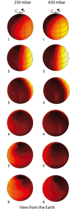
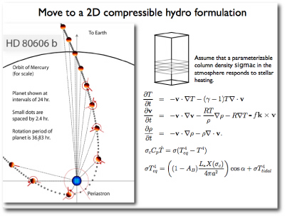
All of the planets observed so far with the Spitzer Space telescope have nearly circular orbits, and hence are in (or are very near) the spin-synchronous state. We’re waiting to hear the results of our Spitzer GO-4 application to observe the highly eccentric planet HD 80606b, during an upcoming ‘606 day. If our observing proposal gets a thumbs-up, it’ll dramatically broaden the range of conditions under which planets have been observed. Very shortly, I’ll be posting the results of calculations that Jonathan Langton and I have been doing which predict what the light curve of HD 80606 should look like during the periastron passage in the various Spitzer bands. Here’s a sneak preview of how the temperature distribution on the planet might evolve over a 36-hour period as seen from a direction consistent with our line of sight from the Earth:

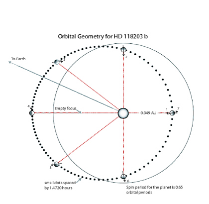
In looking over the latest officially published additions to the catalog of extrasolar planets, I noticed that there’s a very interesting object — HD 118203b — that straddles the extremes of the circular hot Jupiters and the ultra-eccentric HD 80606b. This planet was discovered in 2005 by the Swiss Team, has an orbital period of 6.13 days, a mass at least twice that of Jupiter, and a well-determined eccentricity, e=0.3. HD 118203b therefore won’t be spin-synchronous. Rather, as is also the case with HD 80606b (see the diagram here), it’ll have been forced into a state of pseudo-synchronous rotation, in which it does its best to keep one face toward the star during the periastron passage. Its day should be 64.8% as long as its year:

Higher resolution .eps version here.

Which raises a rather interesting question: Why is HD 118203’s eccentricity so high?

Assuming that the planet has a similar structure to Jupiter, the equations of tidal dissipation (see here for a discussion) indicate that the planet’s orbit should circularize in a mere 10-20 million years. This time scale is surprisingly short because the parent star is a subgiant with a radius ~1.5 times larger than the Sun. Something must be exerting a very strong perturbation to keep this planet’s e up.

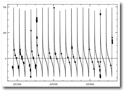
In their discovery paper, Da Silva et al remark that the residuals around the best 1-planet Keplerian fit to the data are very large. It’s quite straightforward to verify this with the downloadable Systemic console (try it!) Da Silva and company were able to improve their fit by including a linear drift of 49.7 meters per second with their one-planet model. This corresponds to adding the effect of an outer planet that has been observed for only a small part of a single orbit. (The 43 published velocities span a period of 1.1 years.) They speculate that an outer as-yet-uncharacterized planet provides the gravitational perturbation that maintains the high eccentricity for the inner planet.

Last year, Fred Adams and I wrote a computer code (see these papers 1, 2) that includes the effect of general relativistic corrections on long-term planet-planet gravitational interactions. It’s easy to use this program to calculate what the long-term influences of various companion planets would have on HD 118203 b’s eccentricity. I ran a few trial cases, and quickly found that the interactions produced by companions that also provide the observed linear drift in the radial velocities don’t seem to be strong enough to explain HD 118203b’s high eccentricity. Could there be another explanation?

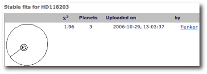
This is the sort of situation where the collaborative systemic back-end is extremely useful. I had a look at the stable fits that have been submitted so far for HD 118203. The best stable, self-consistent fit was uploaded back in October by the user Flanker, and has a reduced chi-square statistic of 1.96:

null.

This fit might point in an interesting direction for some further inquiry. Instead of using a linear trend to soak up the residuals to the one-planet fit, Flanker added two additional planets. One of the planets has a mass of 0.3 Jupiter masses and is orbiting with a period of 15 days. Its periapse is nearly aligned with the periapse of the inner planet. The resulting short-period secular interaction may well be strong enough to keep the eccentricity of the innermost planet high in the face of tidal dissipation. Flanker’s model also contains an outer planet with an orbital period of 244 days and a minimum mass 0.6 times that of Jupiter.

I think it’s worthwhile to explore additional models for this system that contain planets with short enough periods to intereact strongly with the 6.13 day planet. If the perturbing body has a relatively short-period orbit, then its presence will not be hard to verify with additional radial velocity observations of the star. And also, if Spitzer’s cryogen holds out, HD 118203b might be a very interesting target for a full-phase campaign.

Bootstrap

Image Source.

Stefano and Eugenio have been making quite a bit of development progress on the downloadable systemic console. A new version of the console (available for beta testing on the systemic backend) is now capable of providing an estimate of the uncertainties on the orbital elements associated with a fit to a particular data set.

Radial velocity data don’t provide an exact determination of planetary orbits. The most obvious shortcoming is that Keplerian orbital fits can’t determine the inclination of the planetary orbits, and so for a given system, we’re only able to measure then mass of the planet multiplied by the sine of the unknown inclination angle. Furthermore, the stellar radial velocity signal created by a planetary system is corrupted by astrophysical noise introduced by the parent star, as well as by noise introduced during the measurement process here on Earth.

Determination of the true uncertainties in a planetary orbital model is a subtle problem (for more detail, see Eric Ford‘s recent work in this area). As a first straightforward step, we’ve implemented the so-called “bootstrap” method of error estimation into the console. The bootstrap works by taking the original data set, and then successively redrawing time + velocity + uncertainties triples from the data with replacement. This procedure creates alternate realizations of the original data set in which some of the original measurements appear more than once, and in which some don’t appear at all. The best-fit parameters obtained by the console are then used as a starting guess to fit the bootstraped data sets. The standard deviations measured from the distributions of orbital elements thus obtained give error estimates for the parameters of the original fit.

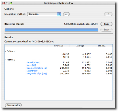
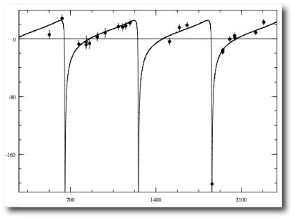
The bootstrap routine is menu-accessed, and is simple to use. First, create a fit to a dataset. In the example just below, I’ve fitted to the data for HD 80606:

Once the fit has been polished, the bootstrap can be run. In the default configuration it uses Keplerian fitting and does 100 trials.

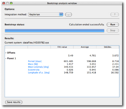
HD 80606 has been observed for nearly 20 orbital periods, and velocities have been obtained at a wide variety of orbital phases. As a result, the orbit is very well constrained. The bootstrap indicates that the uncertainty on the e=0.932 eccentricity is only 0.003. For other systems, such as hd 20782, which also seems to have a high eccentricity:

the uncertainty on the parameters is much larger:

Give the routine a try! In upcoming posts, we’ll talk more about how uncertainty estimates will be incorporated into the planetary catalogs on the backend.

Impact!

Image Source.

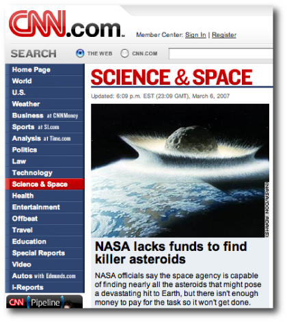
The news out of the Planetary Defense Conference is that NASA has the ability to locate all the potentially dangerous asteroids in our solar system by the year 2020, but that the cash to carry out the project is not currently forthcoming.

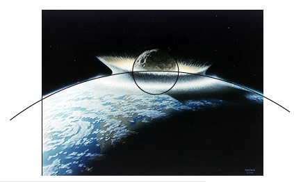
CNN and many other news outlets carried the story, along with a dramatic artist’s rendition of an asteroid striking the Earth.

That’s a rather large asteroid.

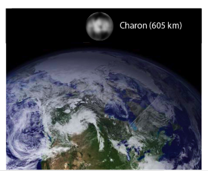
Measuring the circumscribed circles, it appears that the impacting body is 1/10th the Earth’s diameter, or approximately 600 km in radius. A bolide of this magnitude would currently rank as the ~25th largest object in the solar system, larger than Uranus’s moon Umbriel (584 km radius), smaller than Saturn’s moon Iapetus (736 km in radius), and nearly exactly the same size as Pluto’s moon Charon (606 km in radius). Ceres, the largest object in the main asteroid belt, by contrast, has a radius of ~475 km.

Based on the location of the late-afternoon catastrophe relative to the day-night terminator, the impactor seems to have had an orbit that was highly inclined relative to the solar system’s angular momentum plane. Perhaps it was undergoing Jupiter-driven Kozai oscillations prior to striking the Earth.

The last impact of the magnitude shown in the illustration was probably the Moon-forming impact ~4.4 Billion years ago, in which a Mars-sized body struck the Earth. Kevin Zahnle of the NASA Ames Research Center has estimated the distribution of giant impacts after the Moon-forming event. It’s likely that the largest strikes were by bodies with roughly half the radius of the object shown in the above picture.

The consequences of even a 300 km object hitting the Earth are severe. Such an impact is energetic enough to entirely vaporize the Earth’s oceans and create a temporary rock-vapor atmosphere with a surface pressure of ~100 bars. For a period of several months to a few years, the Earth would radiate with a temperature of ~2000 Kelvin — hot enough to glow brightly in the visible region of the spectrum. And depressingly, our planet would be fully sterilized by the event.

This week’s crop

Image Source.

The year 2007 is off to a reasonably good start. Three more planets were announced by the Geneva Planet Search team at a conference in Chile, bringing the total planet crop for ’07 up to seven.

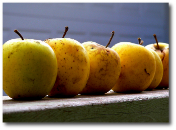
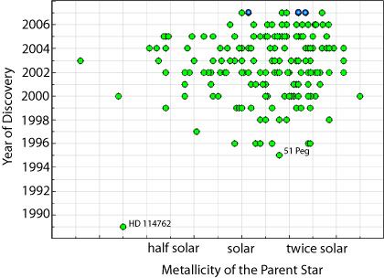
The rate of planet discovery, however, has definitely leveled off. For the past four years, the detection rate has remained fixed at 26 new planets per year. The low-hanging fruit — the 51 Pegs, the 47 Ursae Majorii, the Upsilon Andromedaes — have all been harvested from the bright nearby stars, and increasingly extractive methods are being brought to bear. Transits are starting to contribute significantly to the overall detection rate. Radial velocity is pushing to planets with progressively lower masses. Surveys such as N2K are rapidly screening metal-rich stars that have high a-priori probabilities for harboring readily detectable planets. The neccessity of finding more planets is driving up the average metallicity of the known planet-bearing stars:

The three new planets, HD 100777b, HD 190647b, and HD 221287b are quite ordinary as far as extrasolar planets go. They all have masses somewhat greater than Jupiter, and they all take more than a year to orbit their parent stars. Their discovery seems not to have registered with the news media:

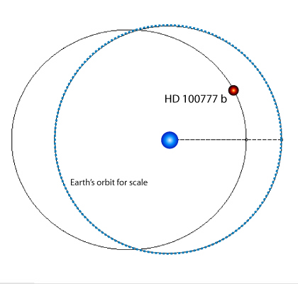
HD 100777 b, however, is actually deserving of some attention. Its orbital period of 383.7 days places it squarely in the habitable zone of its parent star. The eccentricity, e=0.36, is fairly high, and likely leads to interesting seasonal effects in the atmosphere of the planet.

HD 100777 b lies a regime where we expect to see white water clouds forming in the visible atmosphere. The planet is probably very reflective in the optical region of the spectrum (quite unlike the hot Jupiters, which are likely cloud-free, and which are known to absorb almost all of the starlight that strikes them). Convection of interior heat to the surface of HD 100777b is almost certainly driving collossal thunderstorms, and the atmospheric disturbances created by the thunderstorms likely feed giant vortical storms similar to Jupiter’s great red spot.

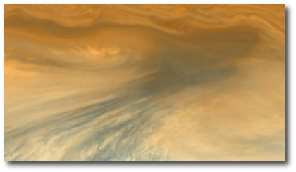
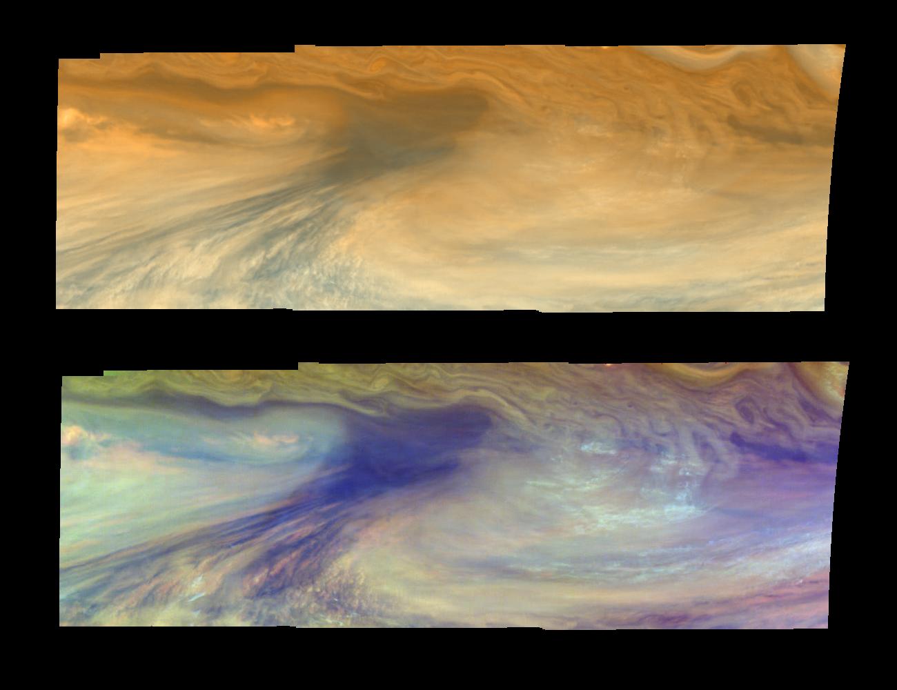
It’s also possible that the atmosphere is much clearer in regions where air wrung dry by rainfall is downwelling. This phenomenon occurs on Jupiter, where highly transparent patches occur over several percent of the Jovian surface:

Image Source.

The Galileo entry probe went right into one of these regions, and sampled very dry air. On HD 100777, the regions of high atmospheric transparency will probably preferentially absorb red and green light (as a result of Rayleigh scattering of incoming photons). The surface, then, in the vicinity of a downwelling region may look something like this:

flyby

Image: NASA New Horizons Spacecraft (false color by oklo).

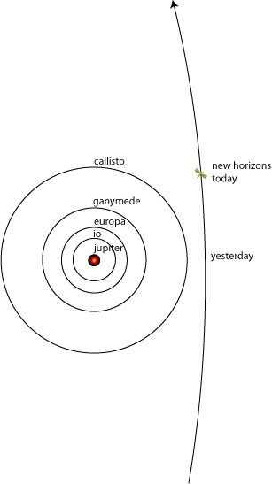
One day, one hour, and nine minutes ago, the New Horizons spacecraft sailed flawlessly through its closest approach to Jupiter. A day later, Jupiter still looms large in New Horizon’s field of view, with an angular size more than five times greater than the size of the full moon in our sky.

Jupiter, during its 4.5 billion year history, has been visited by at least seven other probes. Pioneer 10, Pioneer 11, Voyager 1, Voyager 2, Ulysses, Galileo, and Cassini have all successfully made the journey. This latest encounter was buried beneath the news of a 500-point drop in the Dow Jones Industrial Average. The flyby, in fact, hasn’t even made it onto the Astronomy Picture of the Day!

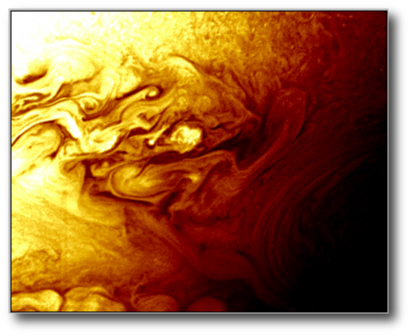
A decade ago, many of the metal atoms in the New Horizons spacecraft were still buried in the Earth’s crust. A bit more than a year ago, the assembled spacecraft was flown, in a sealed pressurized container, to Cape Canaveral for launch. All through the past several weeks, it’s been taking pictures of the Jovian system. Most of the data will be radioed back to Earth over the coming months. The image above was taken on Monday, and shows a Von Karman vortex sheet trailing away from the Little Red Spot, currently the second-largest storm in the Solar System.

In a sense, the Jupiter encounter was mostly utilitarian. It boosted the spacecraft’s heliocentric velocity (at the expense of Jupiter’s orbital energy) and cut down the travel time to Pluto.

The next scheduled mission to Jupiter is Juno, the Jupiter Polar Orbiter, which is scheduled to arrive at the Jovian system in 2016.

spectra

Image Source.

So, uhh, yeah, the oklo blog went through a dry spell with no posts last week. This was primarily a consequence of the fact that Spitzer GO-4 proposals were due last Friday. I teamed up with Drake Deming of GSFC and UCSC physics grad student Jonathan Langton to propose a 30-hour observation of HD 80606b during the ‘606 day that’ll occur next November 20th. In an upcoming article, I’ll be pushing the reasons why we’re really excited about the possibility of observing HD 80606 b during its big periastron swing.

The Spitzer Space Telescope has turned out to be a regular wellspring of exo-planet results. It’s providing very interesting and often surprising constraints on the weather conditions at the surfaces of the hot Jupiters, and another big new result was announced today. Three different teams released the first-ever observations of emergent infrared spectra from two observational runs on HD 189733 and HD 209458.

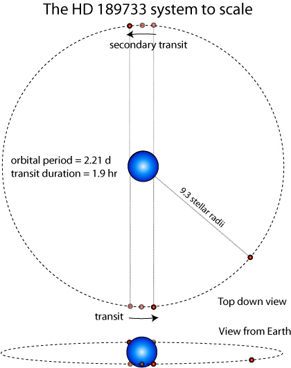
The transiting planet HD 189733 b was discovered by the Swiss team in 2005. Of the fourteen known transiting planets, HD 189733 b is the best-suited for detailed follow-up observations. The parent star lies only 19 parsecs away, the orbital period is a skimpy 2.1 days, and the 1.15 Jupiter-mass planet has a radius fully 15% the size of the primary star’s radius. Like the other transiting systems, the planet, the orbit, and the star can all be drawn completely to scale on a “saved for web” diagram that’s only 420 pixels across:


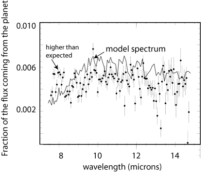
Grillmair et al.’s Spitzer spectrum of HD 189733 was obtained with 12 hours of observation, in which the brightness of the star at infrared wavelengths between 7 and 14 microns is compared in and out of the secondary transit:

The observed flux distribution from the planet is nearly completely flat as a function of wavelength! Models of the atmospheres of hot Jupiters had all predicted that the presence of water vapor in the planetary atmosphere would lead to a prominent absorption feature at ~8 microns. No hint of the predicted dip was seen. The overall amount of infrared light coming from the planet during the secondary transit indicates that heat is probably being efficiently redistributed between the day and night sides of the planet.

A Nature paper by Jeremy Richardson and collaborators reported a very similar result for HD 209458 b. Their spectrum runs between 7.5 and 13.2 microns, is similarly devoid of absorption features, and also suggests a modest day-night temperature difference.

So how to interpret these results? One possibility is that the lack of absorption lines is caused by a high, uniformly emitting cloud layer, perhaps made of silicate grains. A problem with this interpretation, however, is that the cloud decks would have to be extremely dark and unreflective in the optical. Hot Jupiters absorb nearly 95% of the radiation that they receive from their parent stars. Another possibility, put forward by Jonathan Fortney, is that the atmospheres of these planets are isothermal down to large optical depths. Because we can’t actually see to a hotter underlying layer, there’s no mechanism for deep absorption lines to form.

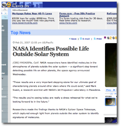
And finally, another, rather startling, interpretation of the results was offered several hours ago by CBS News:

Image Source.

The exoplanet prediction market

Image Source.

At first glance, the market capitalization of the Chicago Board Options Exchange, and the list of astronomers active in the field of extrasolar planets would appear to have nothing to do with one another. These two disparate entities are connected, however, by the fact that they’ve both undergone explosive growth over the past decade, and both are continuing to grow. They signify highly significant societal trends.

I think it’s safe to predict that in 25 years, the market for financial derivatives, and the level of economic activity associated with exoplanets will both be far larger than they are now. It’s interesting to ask, will there be an unanticipated co-mingling between the two? And if so, how will it occur?

One very realistic possibility is the development of an exoplanet prediction market, in which securities are issued based on particular fundamental questions involving the distribution of planets in the galaxy. Imagine, for example, that you’re an astronomer planning to devote a large chunk of your career to an all-or-nothing attempt to characterize the terrestrial planet system orbiting Alpha Centauri B. In the presence of a liquid, well-regulated exoplanet prediction market, you could literally (and figuratively) hedge your investment of effort by taking out a short position on a security that pays out on demonstration of an Earth-mass planet orbiting any of the three stars in Alpha Centauri.

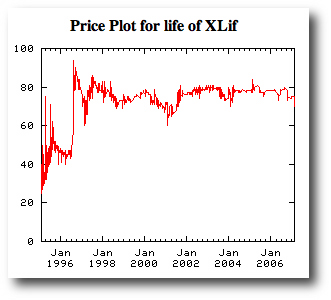
Prediction markets have been adopted in a very wide range of contexts, ranging from opening weekend grosses for big-budget movies, to forecasts of printer sales, to the results of presidential elections. A highly readable overview of these markets by Justin Wolfers (who was featured last week in the New York Times) and Eric Zitzewitz of the University of Pennsylvania is available here as a .pdf file. The ideosphere site contains a wide variety of markets (trading in synthetic currency) and includes securities directly relevant big-picture questions in physics, astronomy and space exploration. Here’s the price chart for the Xlif claim,

which pays out a lump-sum of 100 currency units if the following claim is found to be true:

Evidence of Extraterrestrial Life, fossils, or remains will be found by 12/31/2050. Dead or extinct extraterrestrial Life counts, but contamination by human spacecraft doesn’t count. (Life engineered or created by humans doesn’t count.) The Life must have been at least 10,000 miles from the surface of the Earth. If Earth bacteria have somehow got to another planet and thrived, it counts, as long as the transportation wasn’t by human space activities.

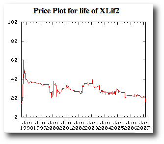
It’s very interesting to compare the bullish current Xlif price quote of 72 with the far more bearish sentiment on Xlif2, which is currently trading at an all-time low of 17,

and which pays out if “extraterrestrial intelligent life is found prior to 2050”, and more specifically,

Terrestrial-origin entities (e.g. colonists, biological constructs, computational constructs) whose predecessors left earth after 1900 do not satisfy this claim. If the intelligence of the ET is not obvious, the primary judging criteria will be either a significant level of technological sophistication (e.g. radio transmitting capability) or conceptual abstraction (e.g. basic mathematical ability). Radio signals received or similar tell-tale signs of intelligence (e.g. archeological discoveries) detected and accepted by scientific consensus as originating from intelligent extraterrestrials would satisfy the claim even if not completely understood by the claim judging date.

Recently, open-source software has been released that makes it straightforward to set up a prediction market. We’ll soon have the world’s first exoplanet stock market up and running right here at oklo.org. In the meantime, feel free to submit specific claims (in the comments section for this post) that might lend themselves to securitization…

glow

Image Source.

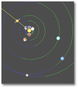
Saturn reached opposition yesterday, marking the moment in our yearly orbit when the Earth draws closest to the massive ringed giant. At midnight, Saturn is currently the only planet visible in the sky. It’s an odd feeling to stare at the bright unresolved spot of light that encompasses the planet, the rings, and the moons into a tiny golden point, and to know that Cassini, our robot emissary, is actually out there, almost a billion miles away, taking photograph after photograph, and radioing them back to a mere mouse click away.

Schematic image of the solar system on 2/11/2007 created at Solar System Live.

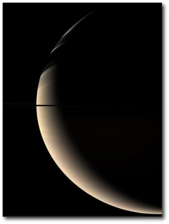
Saturn and its rings are good reflectors of light, but nevertheless, in the vicinity of the planet, the glare is far from overwhelming. The ambient light levels are only a bit more than 1% that of a bright summer day on Earth. It would be easy to stare at the crisply defined terminator marking the day-night boundary on the planet and the arcs of black shadow cast by the rings. On the Cassini website, there are many views that show the planet as it would appear to human eyes.

Image Source.

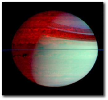
Cassini also has the ability to photograph in the infrared. The following false-color photograph shows visible and infrared images of the planet superimposed. In the infrared, Saturn glows with interior heat — still welling up from the planet’s formation — that illuminates the night from within.

Image Source.

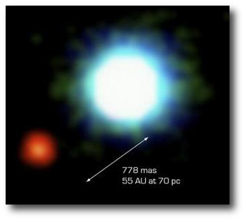
The picture above is not a bad approximation of what a younger more massive planet would look like to the naked eye. 2M1207 b, for example, which seems to have a mass about five times that of Jupiter, is in a 1700-year orbit around a young 25-Jupiter mass brown dwarf. At 1250 Kelvin, 2M1207b is still warm enough to be self-luminous in the visible region of the spectrum. It is also slightly illuminated by the light of its companion (whose ~2500K surface is intrinsically 100 times more luminous.) Methane absorption and Rayleigh scattering of incident light in 2M1207 b’s atmosphere likely give the weak crescent a bluish-green hue.

Image Source.

Lonely Planet Guide to the Hyades

Image Source.

It’s been a hectic week, and now that it’s February, my New Year’s resolution to write 2-3 posts per week managed to lose its shaky option on my priorities.

Eugenio stopped by my office this afternoon to outline his latest code developments for the console. He’s mostly finished implementing a Bulirsch-Stoer integrator. Once this algorithm is tested and operational, it will produce very significant speed-ups for the fitting and the stability analysis of tough multiple-planet systems such as 55 Cancri and GJ 876. Then it’ll be on to a rollout of the bootstrap method for computing uncertainties for the orbital elements in the planetary fits.

“So did you see the new planet?” he asked.

“Huh?” I hadn’t heard anything about it.

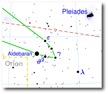
Turns out that Bunei Sato and his collaborators have detected a periodic radial velocity variation for the star Epsilon Tauri. Their preprint is on the Astrophysical Journal’s website, but it doesn’t seem to have hit the preprint server yet. This star is a prominent member of the nearby Hyades cluster, and is easily visible to the naked eye as part of the well-known “V”-shaped asterism near Aldeberan in the sky.

Image Source.

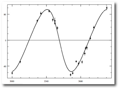
Eps Tau is bright enough to have garnered 40 different names in the Simbad catalog, and it’s now listed in the console menu and on the systemic backend as HD 28305. This is one of the most straightforward radial velocity datasets that you’ll come across, and thus makes a good system for first-time users to fit. A few debonair moves with the downloadable console conjure up a model planet with a period of 594 days, an orbital eccentricity e=0.15, and a minimum mass 7.6 times that of Jupiter:

Epsilon Tauri is one of the four stars in the Hyades that are currently nearing the end of their lives and are evolving through the red giant phase. It’s 14 times larger than the Sun, and it’s luminosity is 97 times the solar value. It weighs in at 2.7 solar masses, making it the most massive star known to harbor a planet.

So what’s the story? The Hyades are a metal-rich cluster. One would naively expect that the supersolar composition of the precursor star-forming giant molecular cloud would have lead to a large fraction of the cluster members harboring readily detectable planets. It’s also true that stars somewhat more massive than the Sun should harbor a higher-than-average fraction of giant planets. Eps Tauri scores on both counts.

[Note: John Johnson‘s thesis work at UC Berkeley and Bunei Sato’s RV survey are both capable of providing observational support for the hypothesis of a positive correlation between the detectable presence of a planet and the mass of the parent star. See talk #1 on the Systemic Resources page for more details.]

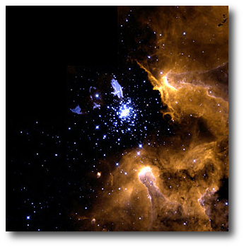
Young Cluster NGC 3603, Source: NASA

It’s important to keep in mind, however, that a cluster environment will have a strong effect on giant planet formation. Currently, the Hyades are 600 million years old, and the cluster has lost a large fraction of its O.G.s to the general galactic field through the process of dynamical escape. If we extrapolate back to the cluster’s early days, we find that the Hyades would have resembled the Pleiades 500 million years ago, and would have looked like the Orion Nebular Cluster during the first few million years of its existence.

The UV radiation environment in the original Hyades cluster was fierce. The protostellar disks of the individual Hyads were likely photoevaporated before the growing planetary cores were able to reach the runaway gas accretion phase that gives rise to Jupiter-mass planets (see our paper on this topic). When we get the full inventory of planets in the Hyades, I think we’ll find plenty of Neptunes and terrestrial planets, but almost nothing in the Jovian range. Indeed, work by Bill Cochran and the Texas RV group has demonstrated that the Hyades are generally deficient in massive planets.

My guess is that Epsilon Tauri b is an example of a planet that formed through the gravitational instability mechanism. Gravitational instability should generally produce more massive planets (e.g. HIP 75458 b, and HD 168443 b and c) and its efficacy will be little-affected by UV radiation from neighboring stars. It likely occurs once per every several hundred stars that are formed, and so it’s perfectly reasonable that there’s one star in the Hyades that has a planet formed via the GI mechanism.

For more information, this series: 1, 2, 3, 4, 5, 6, and 7
of oklo posts compares and contrasts the gravitational instability and core accretion theories for giant planet formation.

a bunch of cool new stuff

Image Source.

Stefano and Eugenio have both been working hard on the systemic console and backend, and as a result of their efforts, we’re now able to roll out a number of new features.

The backend now features a systemic wiki in which users can collaborate on a wide variety of writing projects related to systemic in particular and extrasolar planets in general. Features include discussion pages for individual systems, the framework for a comprehensive console and backend manual, and an exoplanetary news wire. Our first news service is being provided by Mike Valdez, who combs astro-ph every day and extracts any new preprints that are germane to the those interested in exoplanets. Stefano wrote the code from scratch, so there are endless possibilites for customization. Give it a try.

On the console front, Eugenio has aggregated a uniform listing of the literature sources of all of the radial velocity data sets provided by the console. This information is in a file vels_list.txt, which is now included in the systemic.zip package. If you are using the console for scientific research that you intend to publish, it’s now a snap to get the correct citations for any of the individual systems included on the console.

Many users have expressed interest in what our own solar system would look like to a dedicated radial velocity observer on another star. Eugenio has put together an expansion pack that contains 17 manufactured data sets based on the Solar System. A second expansion pack contains an analogous set of manufactured data sets for various plausible configurations of planets orbiting Alpha Centauri A and B. Both are available on the downloads page for the downloadable systemic console.

Check it out!

…and then the clouds lifted

Image Source.

I drove up to Berkeley yesterday to give a talk about my second-favorite planet — HD 80606 b. A good fraction of the keynote slides in the talk were new, and so I wound up spending most of the weekend scrambling to get my story straight and to get the talk together.

Pacing is always tricky the first time that you give a talk on a new topic. You’re supposed to practice your talk before you give it, but It’s hard to get in that recommended hour-long practice session when it’s 2AM the night before, and you’re fading, and there are still four slides to finish making.

Thirty-seven minutes into the talk, it suddenly dawned on me that I’d put together too much material, and so I wound up rifling pretty quickly through the last half of the slides. In an entire career as an academic, I’ve never heard of anyone being unhappy when a talk ended on time rather than going over, so I always wrap things up to come in under the bell no matter what.

Over the weekend, I realized a rather remarkable thing about HD 80606b:

Because of the highly eccentric orbit, there’s quite a bit of tidal energy being deposited inside the planet. This tidal energy source, in fact, likely exceeds the amount of energy that the planet absorbs in the form of radiation from the star. For a tidal quality factor, or Q-value of 300,000, the planet will have an effective temperature at apastron of about 390K. That is right at the boundary where water clouds can form in the planet’s upper atmosphere. If the planet is hotter (that is, if Q is lower than 300,000), then the atmosphere will always be cloud-free, and the visible layers of the surface will have a low albedo. If the planet is cooler (that is, if Q is significantly larger than 300,000), then near apastron, the visible surface will consist of a shroud of highly reflective water clouds.

In either event, during the time surrounding ‘606 day, the atmosphere will be too hot for water clouds, and so the albedo will be low when the planet is close to the star. Therefore, if Q is low, there’ll be a smooth variation in the reflected light from the planet over the course of an orbit. On the other hand, if Q is high, then there’ll be a sharp (and potentially observable) drop in the reflected-light signal as the clouds flash to steam.

[I’ve put the slides from the talk on the systemic resources page.]

300B

Image Source.

The 200-odd extrasolar planets that have been discovered with the radial velocity method are orbiting stars that lie within a few hundred light years of the Sun. The light we now see coming from GJ 876 left that red dwarf back in early August 1991. When you’re in the bars drinking to celebrate the periastron passages of HD 80606 b, it’s easy to forget that last December’s periastron passage actually occurred in September 1817.

By galactic standards, however, a distance of 300 light years is still right next door. For every star within 300 light years of the sun, the Milky Way contains roughly 300,000 additional stars that are farther away. All told, adopting the latest rules on what constitutes a planet, our galaxy likely contains about 300 billion planets, of which perhaps 500 million are hot Jupiters.

Right now, 51 Peg, HD 209458, Upsilon Andromedae, et al. count among the Sun’s local galactic neighbors, but this hasn’t always been the case. The velocity dispersion of stars in the solar neighborhood is ~20 kilometers per second. A kilometer per second is a parsec per million years, which means that in a mere 15 million years, the roster of nearby planets will contain very few familiar names. HD 209458b is transiting now, but in a few hundred thousand years, it’s likely that the line of sight to the system will no longer allow Earthbound observers to watch that dip every 3.5247542 days.

So get out there while there’s still time! Due to a computer glitch, the transitsearch candidates table failed to get its nightly update for the past several nights. I’ve fixed the problem, and the ephemerides are all up to date.

hot and bothered

Image Source.

When an extrasolar planet transits its parent star, we get the opportunity to learn the physical size of the planet by measuring how much of the star’s light is blocked during the occultation. To date, fourteen extrasolar planets have been observed in transit, and the big surprise is that they have a much wider range of sizes than astronomers had predicted.
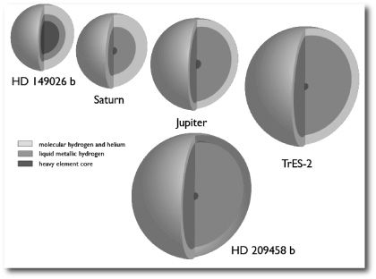
Five for the show

HD 149026 b, for example, is more than 30% smaller in size than one would expect. Its dense, dimunitive stature is thought to stem from a ~70 Earth-mass core of elements that are heavier than the hydrogen and helium that dominate the composition of most of the known extrasolar planets. HD 209458 b, on the other hand, is roughly 30% larger than predicted. The reason for its bloated condition isn’t fully clear, but it’s believed that the planets with larger-than-expected radii are tapping an extra source of internal heat that keeps them eternally buff.

A lot of astronomers are currently interested in the size question for the extrasolar planets, and we’ve written a number of oklo.org posts that cover the subject. [See 1. here, 2. here, 3. here, 4. here, 5. here, 6. here, 7. here, 8. here, and 9. here.]

Josh Winn (MIT) and Matthew Holman (Harvard-Smithsonian CfA) have written a paper that presents an interesting hypothesis for resolving the HD 209458 b radius dilemma. Winn and Holman propose that the planet is caught in a so-called Cassini state, which is a resonance between spin precession and orbital precession. In short, if HD 209458 b is trapped in the “Cassini state 2”, then its spin axis will lie almost in the orbital plane. Like all short-period planets, the planet will spin once per orbit, but it will literally be lying on its side as it circles the parent star. A hot Jupiter in Cassini state 2 will easily experience enough tidal heating to maintain a 30-percent pump.
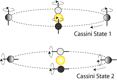
If a planet is in Cassini state 2, then the pattern of illumination on the surface is rather bizarre. At the north and south poles, the parent star rises and sets once per orbital period, and at mid-day passes directly overhead in the sky. This contrasts with the two locations on the equator from which the parent star never rises above the horizon, and the two other spots from which the star never quite sets. Here are two short .avi format animations that help to illustrate the situation. In the first animation, we hover above the point on the equator that receives maximum illumination. In the second animation, we hover above the point on the equator that receives the least illumination.

I’ve been working with UCSC physics graduate student Jonathan Langton to model the surface flows on extrasolar giant planets. As a first research problem, we made simulations of what the surface flows might look like on a planet in Cassini state 2, and compared them with the flows on a planet in Cassini state 1. Jonathan has just had his paper accepted by ApJ Letters. It should show up on astro-ph very shortly, but in the meantime, here’s a link to the .pdf file for the accepted version.

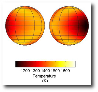
The results of Langton’s simulations are interesting. If the planet is in the standard-issue Cassini state 1, then a steady-state flow-pattern emerges on the planet, with the hottest temperatures occuring eastward of the substellar point, and the coldest region lying near the dawn terminator of the night-side:
If the planet is in Cassini state 2, then Langton’s model shows that a periodic flow pattern emerges which repeats every orbital period. In the figure below, each successive frame is advanced by 1/4th of an orbital period. The top row of images corresponds to an equator-on view, and the bottom row of images corresponds to a pole-on view:
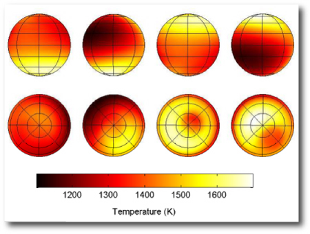
It’s interesting to watch the animations of the temperature flows. Here’s a link to the equatorial view (5.7 MB, .avi format).

Event though the surface flow patterns are quite different in Cassini State 1 and Cassini state 2, the overall light curves as viewed from Earth don’t show much diffence. The figure below shows infrared emissions from the planet over one full rotation period. The blue line shows the Cassini state 1 light curve, the red line shows the Cassini state 2 light curve. These two curves are more similar to eachother than they are to the Cassini state 1 light-curve predicted by Cooper and Showman (2005), who used a different simulation method and a different set of assumptions, and got a larger overall variation in the predicted infrared emission from the planet during the course of an orbit:
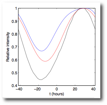
It will be tough to use the Spitzer telescope to reliably distinguish which Cassini State the planet is in.