Visitors to oklo.org may have noticed that the site was down for most of Sunday. I’d been neglecting to update my WordPress installation, which lead to a problem with the database, and a huge load spike for the server. Everything seems stable now, and I’m now flossin’ 2.8.4 inch rims.
In the relatively near future, I will be modernizing some aspects of the look and feel of the site, which will make it more discussion-friendly, and more smoothly slotted into the hum of the outside world. No need to worry, though. We’ll continue to roll ad-free.
I’ve updated the second systemic console tutorial which guides the user through the remarkable Upsilon Andromedae radial velocity data set. The back-end database is getting closer to its relaunch, and the systemic console (version 1.0.97) is freely available for download here.
Read on to work through the tutorial.
Console Tutorial #2 — The Ups and Downs of Ups And
The star Upsilon Andromedae lies roughly 40 light years away in the constellation Andromeda, and (unlike most of the known planet-bearing stars) is bright enough to be visible to the naked eye if you know where to look. Upsilon Andromedae is roughly 2.5 billion years old (about half the age of our Solar System), and is about 30% more massive (and roughly twice as luminous) as the Sun. Because of its relative brightness and proximity, and because it is reasonably similar to the Sun, it was among the original group of 50-odd stars surveyed for planets by Paul Butler and Geoff Marcy using the radial velocity technique. It was also one of the first stars found to be accompanied by an extrasolar planet. More than a decade on, it’s interesting to read the original discovery paper. (See Butler et al. 1997, “Three New 51-Peg Type Planets”, Astrophysical Journal Letters, 474, 115-118).
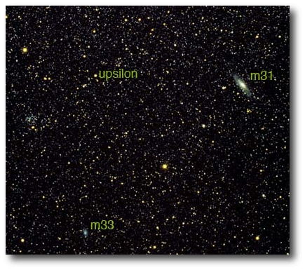
One of the several publicly available Upsilon Andromedae data sets was published by Fischer et al. 2003, and contains 253 individual radial velocity measurements that span more than 15 years of observation. It’s thus capable of giving the systemic console a very informative workout. In this tutorial, we step through the procedure for “discovering” the planets that exist in the Fischer et al. (2003) radial velocity data. We assume that you have already worked through the first tutorial, which analyzed the much less extensive data set for HD 4208, and which introduced the basic concepts that underlie the fitting of orbital models to radial velocity data.
To get started, double-click on the Console.jar icon and let the console’s initialization procedure run its course. When the console is ready for action, click on the system dialog icon (the yellow star symbol near the upper-left-hand corner of the console) and type “UpsAnd” into the text box at the upper-right-hand of the system dialog window. You’ll have a choice between a number of different data sets for Upsilon Andromedae. Because the parent star is so bright and because the planetary system is so interesting, it has been studied by nearly every active team that uses the Doppler velocity method to detect planets. For the tutorial, you’ll be using the first data set in the list. It’s labeled “upsand”.
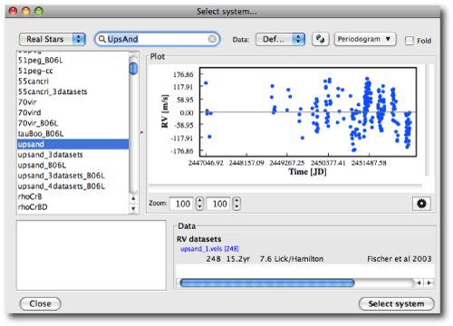
The “upsand” data set was obtained with the venerable 3-meter Shane telescope on Mt. Hamilton. The published reference for the data and important thumbnail statistics (duration, number of observations) are shown in the lower right hand corner of the system dialog window. Click “select system” to load the data into the console, and if prompted, click “OK” to accept the default data set.
Notice how the data-taking rate increased dramatically during the time span that covered the observations. After Upsilon Andromedae was discovered to harbor a multiple-planet system in early 1999, it began to be observed much more frequently. The radial velocity surveys, with their limited budgets of observing time, continually re-balance the conflicting demands of obtaining as many observations as possible of interesting systems, while simultaneously devoting as uniform a coverage as possible to as many different stars as possible. When Upsilon Andromedae proved its worth, it started getting lots of attention.
In the case of the star HD 4208, which was the subject of tutorial #1, it was straightforward to find a decent one-planet fit to the radial velocity data set simply by manipulating the console’s sliders, and then applying a final “polish” to get a best fit. This was possible because the planet accompanying HD 4208 has only been observed for two orbits, and because it is apparently the only large planet orbiting that star. With Upsilon Andromedae, however, the complexity of the radial velocity data set hints at the presence of several significant planets with different periods. To get a foothold, we need to compute a periodogram that tells us which frequencies (that is, which potential planetary periods) are most prevalent in the data. Click the periodogram button near the top-middle of the console. After a moment, a completed, densely-sampled Lomb-Scargle periodogram will appear in its own window:
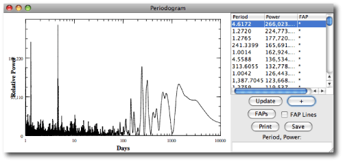
The periodogram indicates that a number of different periodicities are present in the data. The most important peaks are listed to the right of the plot. The higher the power, the more important the peak. In this case, the strongest peak is at 4.617 days. We make the hypothesis that the highest peak is due to a planet, and we therefore activate the first row of orbit sliders (using the button to the far left of the row).

By typing in the box, enter 4.6172 into the period controller for planet #1. Note that if you use the slider, you will have difficulty getting this exact value to appear.
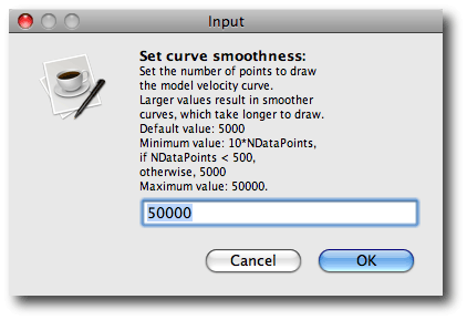
With a 4.617 day period, the full radial velocity plot on the console window becomes totally useless. The prospective planet has executed more than a thousand orbits over the length of time (~15 years) that the star has been observed. First, click on “set curve smoothness” under the options menu, and enter 50,000, the maximum resolution available for plotting:
Then, use the zoom and scroll sliders beneath the plot to focus in on one of the well-sampled regions:
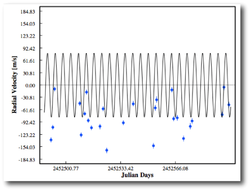
A quick inspection of the excursions of the radial velocities relative to the sinusoidal pattern produced by a single 4.617-day circular orbit suggests that more than one planet may be contributing to the overall radial velocity signal. There are trends in the distribution of points which clearly unfold over periods of hundreds of days and more. Ignore these longer-term trends for the moment, and focus on pinning down the orbit of the 4.617 day planet.
Click on the “Mean Anomaly” line minimization button for planet one:

This automatically varies the mean anomaly (defined at the epoch of the first radial velocity data point) through the full 360 degree range, and selects the value that gives the best fit to the data. The chi-square of the fit drops to something in the neighborhood of 80, and the RMS scatter drops to roughly 60 meters per second.
Next, by clicking on the line minimization buttons for Period, Mass, Mean Anomaly, and Stellar Offset, you can try to improve the one-planet fit. A few cycles of clicking brings the chi-square down to 65.8 (the exact values that you calculate might deviate slightly from this, depending on the particular history of operations that you’ve performed). A final round of improvement can be obtained by sending the Period, Mass, Mean Anomaly, and Stellar Offset parameters to the Levenberg-Marquardt multi-parameter minimization algorithm. You do this by checking the square left hand buttons and then clicking the “polish” button near the top-left of the console.
A good way to display the resulting fit is to “fold” the data by plotting it at the periodicity of the 4.617-d planet. You can do this by selecting “fold to period of planet 1” after clicking on the fold menu button in the upper-right corner of the console.
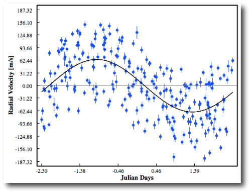
The huge scatter indicates that the resulting model is by no means a satisfactory fit to the data! Upsilon Andromedae definitely seems to be accompanied by a ~0.7 Jupiter mass planet on a 4.167 day orbit, but there is clearly more going on. Indeed, when Paul Butler and his collaborators announced their discovery of the 4.167 d planet in 1997 on the basis of just the first 36 radial velocities, they noted that,
“The 36 velocities show evidence for variability in the gamma velocity of the sine wave on a timescale of about 2 yr with amplitude of 50 meters per second.”
Back in 1997, that was all they could say, but with the large number of additional velocities that have been published since then, we’re in much better shape to figure out what is going on. Indeed, there are several ways that one can proceed to improve the fit. One strategy might be to explore non-zero orbital eccentricities for the 4.167-day planet. (If you’re interested, you can give that a try and verify that non-circular orbits for the inner planet don’t do much to improve the fit.) An alternate, and in this case more profitable, way to proceed is to search for additional planets in the system. To do this, we want to subtract off the radial velocity signal arising from the short-period 4.617 day planet, and look for the remaining periodicities in the system. This is accomplished by clicking on the periodogram of the residuals, or “Res. Periodogram” button at the top of the console. It operates just as advertised, yielding:
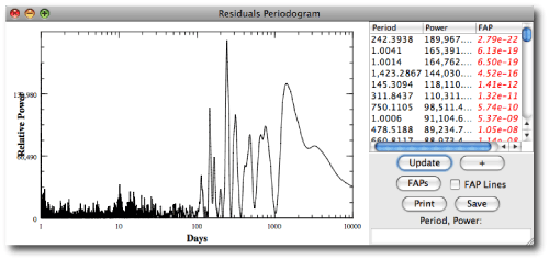
In this periodogram, the strongest peak in the data occurs at 242.394 days, with the another very significant peak falling at ~1423 days. There are also peaks near exactly one day, which are aliases arising from the fact that the star was often observed with a 24-hour night-to-night cadence. Let’s assume that there is a second planet in the system with a 242.394 day period. Activate the second planet, enter the period, and then use the line minimizers to improve the fit (leave the eccentricities of both planets at zero for the moment). After a few rounds of clicking, the two-planet version of the system rolls into a local minimum of parameter space.
The fit can be improved a bit more by polishing with the Levenberg-Marquardt algorithm, but clearly, however, there may be additional bodies contributing to the radial velocity variation of the star. To find what might still be lurking, compute a periodogram of the residuals to the 2-planet fit (by clicking “update” in the residuals periodogram window).
The 242 day peak has been completely eliminated, leaving a single peak at 1290.0 days that contains a lot of power. Activate a third planet with this period, and polish the fit by line minimizations (start with the Mean Anomaly) followed by multi-parameter minimization (polish) using Levenberg-Marquardt.
With three planets on the books, the fit has improved significantly, but is not yet adequate. At this point, one could try to add a fourth planet based on the result of the residuals periodogram. Alternately, one could open the system up to eccentric orbits. To explore eccentricity, pull the eccentricity sliders of the outer two planets up to modest non-zero values (for example e=0.1 for both). Then improve the radial velocity fit with line minimization followed by another application of the Levenberg-Marquardt algorithm.
A successful model of the system has eccentricities of order e=0.27 and e=0.26 for the two outer planets, and the model radial velocity curve really does quite a good job of tracing the observations:
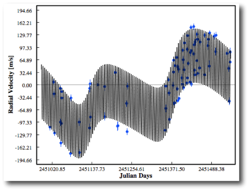
In an upcoming tutorial, we’ll look in more detail at how we can statistically quantify the meaning of “good job”. Here’s a (full-resolution screen-shot of the console) when the currently accepted three-planet model of the system is dialed up on the console.
Note that by using the zoom-in and zoom-out buttons on the orbital view window, you can examine the actual top-down view of the co-planar model system. The arrow button allows you to pop the orbital view out into its own separate window.
