
It’s been unseasonably cold in Santa Cruz. Last night, a freak hailstorm left drifts of icy planetesimals lodged between the leaves of the banana tree outside the bedroom window.
My office, however, is nice and warm. This is because two 2.5 Ghz G5 processors are running mercury.f at full tilt to simulate the formation of habitable planets orbiting low-mass red dwarf stars. The calculations are being done in preparation for Ryan Montgomery’s presentation at AbSciCon in Washington D.C. Two weeks to go.
Two Spheres Within A Sphere Alexander Calder, 1931
Most of the runs have already been carried out using a linux-based beowulf cluster, which is able to run more than 100 individual simulations at once. Each of these simulations starts with 1000 low-mass planetesimals, and calculates the final stages of terrestrial planet formation by allowing the orbiting planetesimals to interact under their mutual gravitational influence. Collisions and ejections gradually winnow the initial swarm down to a few surviving terrestrial mass planets. By doing many simulations, we build up a statistical picture of what the distribution of red dwarf planetary systems should look like.
The desktop computer contains the fastest individual processors to which we have full access. We’ve therefore harnessed it for a single test-case run to investigate the overall sensitivity of our results to the number of initial particles. The processors have spent the last six weeks evolving a system that had an initial distribution of 10,000 small planetesimals. At the projected rate of evolution, it should just manage to finish up just in time. Indeed, if you see Ryan hunched over his laptop at the conference, you’ll know what he’s up to.
John Chambers’ Mercury code (like the Systemic Console in integrator mode) is based on the method of direct summation. At each timestep, each particle in the simulation experiences a gravitational attraction of the form GM/r^2 from every other body in the system. For a 10,000 particle system, that means of order ((10,000)x(9,999))/2=49,995,000 square roots must be computed every timestep (and the actual number is higher, because each timestep consists of a considerable number of substeps). As the number of particles increases, the cost of the calculation increases as the number of particles squared. Our 10,000 particle simulation is 100 times more expensive than the 1,000 particle production runs, and thus pushes the limits of what we can currently readily do.
Many problems in gravitational N-body dynamics can be solved without resorting to direct summation. In essence, this is because to a high degree of approximation, the gravitational attraction from distant particles depends only on the the rough location and total mass of the distant particles. One gets nearly the same result by lumping distant particles into a single, equivalent, large-mass particle:
Using clever variations of this basic idea, one can speed up an N-body (or equivalently, an SPH) calculation enormously. Competitive N-body codes for large-N problems, such as the collisions of galaxies or the formation of structure in the early universe, generally scale as N log(N). For large N, the difference between N^2 and N log(N) is profound. With a million particles, for example, an N log(N) calculation is a cool 72,382 times faster than the brute-force N^2 approach.
One might ask, is there a way to further speed up the computation of the gravitational forces so that finding the accelerations becomes an order N process?
Remarkably, an order-N computational N-body method was employed by Erik Holmberg of the Lund Observatory in Sweden in 1941. Instead of integrating the equations of motion with a computer, Holmberg modeled a two-dimensional system of gravitating particles as an actual physical distribution of movable light bulbs laid out on a gridded sheet of dark paper! Because the intensity of light from a point source diminishes as 1/r^2, one can directly relate the intensity of the light at a particular spot to the gravitational acceleration. The order-N^2 process of computing the gravitational force on a given particle from all of the other particles reduces to a measurement of the total intensity of light in two perpendicular directions using a photocell and a galvanometer. Since one set of measurements is required for the location of each light bulb, the method scales as N. Here is a link to Holmberg’s paper. It’s one of my all-time favorites.
With his analog method for computing the net gravitational acceleration on each of his light bulb “point masses”, Holmberg could compute the change in trajectories which would occur over a time interval using a simple integration scheme such as Euler’s method. A timestep would then be completed by moving all of the light bulbs to their updated positions, at which point a new estimate of the gravitational acceleration could be made. Holmberg’s scheme allowed him to gain a better understanding of important aspects of the dynamics of close encounters between disk galaxies, including the phenomena of orbital decay and the formation of tidal tails:
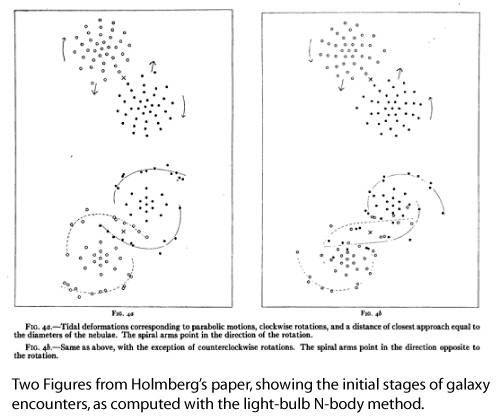
There is an interesting lesson to be drawn. Use of an analog method reduces an N^2 direct summation computation to order N, foreshadowing a time when quantum computation will similarly reduce the computational time for direct summation from N^2 to N. Until that time, however, the light-bulb method beats all others as the number of particles approaches an arbitrarily large value.
In honor of analog methods, here’s a home-made mpeg-4 stop-action animation of a peppercorn orbiting a kumquat in an ellipse with e=0.90. (Try this version if the other one loads a screen of gibberish).
 .
.