

Image Source.
With the verdict in on Pluto, we here at oklo.org will have to revert to sober, scientifically rigorous posts on extrasolar planetary systems to keep our readership and ad rates up. And as soon as I can figure out how to make WordPress launch those “swing for the fences” pop-ups from our site, we’ll be increasing our revenue stream even more.
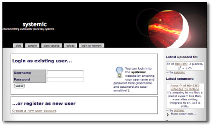
American Scientist has just published my article on planet formation and extrasolar planets in their September/October issue. The article wraps up with a description of the systemic console, and the systemic collaborative research project. If you’re an American Scientist reader visiting oklo.org for the first time, welcome aboard!
Several posts back, I put up a brief description of the immediate goals of the Systemic collaboration:
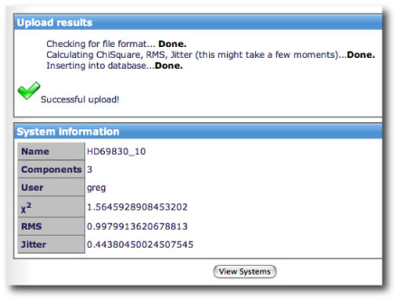
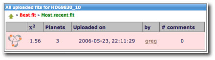
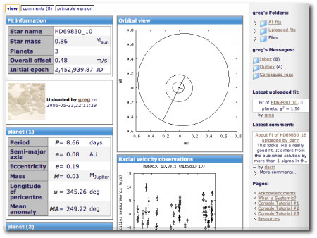
The Systemic collaboration is proceeding in three steps. In the first step, which is ongoing, we’ve been gathering all of the radial velocity data that have been published for known planet-bearing stars. These data sets are included in the downloadable systemic console, and the systemic back-end allows participants to upload their own planetary fits to this data. We want to use the data to create a uniform catalog of known planetary systems.
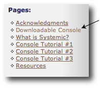
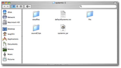
In the second and third phases of the systemic project, we’ll be studying synthetic data sets that have been produced using our own algorithms. “Systemic Jr.” will launch at the beginning of September, and will contain 100 synthetic data sets, four of which will be special challenge systems. The Systemic Challenge, sponsored by Sky and Telescope will be explained in more detail, and will be available at a link on their website. The challenge systems will be released on September 3, 10, 17, and 24, along with a specific set of contest rules. The first person to crack each of these systems will recieve a paperback edition of the Millennium Star Atlas (a $149.95 value). In order to prepare for the contests, go ahead and download a copy of the systemic console, and work through tutorials one, two, and three. A full technical manual for the console is in the works, and will be ready for download quite soon.
Later this Fall, when Systemic Jr. wraps up, we’ll launch the full Systemic simulation. A lot more on this will be posted in the weeks ahead. Our overall goal is to obtain an improved statistical characterization of the galactic planetary census.
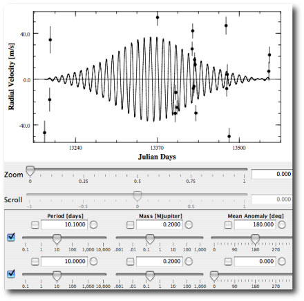
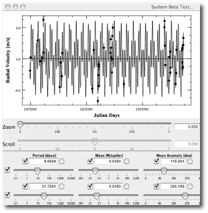
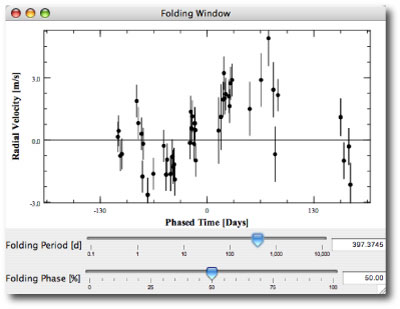
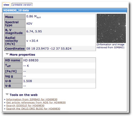
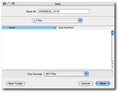
The most interesting serious-planet news from the past week has been the paper by the Geneva Extrasolar Planet Search Team that releases an updated radial velocity data set for the nearby solar-type star Mu Arae (also known as HD 160691). As discussed in this post, the console can be used to quickly uncover and characterize the orbits of the four planets that have been announced for the system.
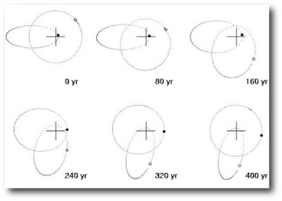
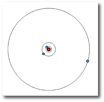
The mu Arae system is remarkable because the two middle planets (with periods P~300 days, planet “d”, and P~640 days, planet “b”) experience strong mutual gravitational interactions during the 5-year time period that the system has been observed. The presence of strong interactions indicates that a model for the system built from independant Keplerian orbits cannot provide a fully realistic fit to the system. In order to build a fully self-consistent fit, one must find an N-body model. The systemic console has this ability, which is enabled whenever the “integrate” box is checked.
N-body integrations are much more time-consuming to compute than simple evaluations of Keplerian fitting functions. The performance of the console thus slows down considerably when integration is enabled. (Note also, that this post now becomes a bit technical. If it sounds like gibberish, you can either skim the next few paragraphs, or, better yet, work through the tutorials on the use of the console.)


