Image Source.

The third Systemic Challenge closed to entries on Friday, and I’ve gone through and evaluated the submitted fits. The results were very encouraging. Eight out of twenty-five submissions corresponded to both the correct orbital configuration and the correct number of planets in the underlying dynamical model.

For challenge 003, we looked to our own solar system for inspiration, and tapped the four Gallilean satellites of Jupiter. Eugenio writes:

The system is a scaled-up version of Jupiter and the four Galilean satellites. To generate the model, I first set the central mass to 1 solar mass. The (astrocentric) period of Callisto was set to 365.25 days, and I required that the mass and (astrocentric) period ratios in the system would remain the same. Here’s the resulting model (using Jacobi elements, with i~88 deg):

Among the eight entries that got both the total number of planets and their periods correct, there was a fair amount of variation among fits that had nearly equivalent values for the chi-square statistic. Chuck Smith (among others) turned in a configuration that bears a very strong resemblance to the actual input system. The four planets in his fit all have nearly circular orbits:

and the resulting radial velocity curve does a very good job of running through the data, with a chi-square value for the integrated fit equal to 1.1005:

A number of other users turned in very similar configurations.

Because of random measurement errors in the data, the true underlying planetary configuration will not necessarily provide the best fit to a given set of radial velocity observations. Often, a better fit can be found for a configuration that is different from the system that generated the data. Steve Undy, for example, achieved a slightly lower chi-square value for his fit by giving a very significant eccentricity to his “Europa”:

The winner of the contest, however, was Eric Diaz, who submitted a 6-planet fit that achieves an integrated chi-square value of 1.04. In addition to the four planets that are actually present in the model, Eric added small planets with periods of 1.06 days and 18.11 days. These objects soaked up some of the residual noise in the fit, allowing for a lower chi-square value, and a copy of the Sky and Telescope star atlas. Nice job Eric!

The contest raises some interesting issues. First, at what point should one stop adding planets to a fit? The chi-square statistic penalizes the inclusion of additional free parameters in a fit, but it’s clear that chi-square can nearly always be lowered by adding additional small bodies to the fit. Second, its very encouraging to see that subtle, but substantially non-interacting systems can be pulled out of radial velocity data sets. In this system, the masses of the planets are small enough so that their dynamical interactions with eachother are not significant over the time-frame that the system is observed. This is in stark contrast to systems such as GJ 876 and 55 Cancri where it is vital to take interactions into account (by fitting with the integrate button clicked on). Finally, I think that we’ll soon see examples of the 1:2:4 Laplace resonance as competitive fits within the existing catalog of radial velocity data sets on the systemic backend.

Image Source.

Guillermo Torres of the CfA recently posted an interesting article on astro-ph in which he takes a detailed look at the planet-bearing binary star system Gamma Cephei.

Gamma Cephei has a long history in the planet-hunting community. In 1988, Campbell, Walker and Yang published radial velocity measurements which show that Gamma Cephei harbors a dim stellar-mass companion with a period of decades. More provocatively, they also noted that the star’s radial velocity curve shows a periodicity consistent with the presence of a Jupiter-mass object in a ~2.5 year orbit around the primary star. In a 1992 paper, however, they adopted a cautious interpretation of their dataset, and argued that the observed variations were likely due to line-profile distortions caused by spots on the stellar surface. From their abstract:

In 1988 Gamma Cep was reported as a single-line, long-period spectroscopic binary with short-term periodic (P = 2.7 yr) residuals which might be caused by a Jupiter-mass companion. Eleven years of data now give a 2.52 yr (K = 27 m/s) period and an indeterminate spectroscopic binary period of not less than 30 yr. While binary motion induced by a Jupiter-mass companion could still explain the periodic residuals, Gamma Cep is almost certainly a velocity variable yellow giant because both the spetrum and (R – I) color indices are typical of luminosity class III. T eff and the trigonometric parallax give 5.8 solar radii independently.

In October 1995, 51 Peg b was announced, and exoplanet research was off to the races. The Walker team, with their futuristic RV surveys had seemingly come close to success, but had not managed to snag the cigar.

In the Fall of 2002, however, the planetary interpretation for the Gamma Cephei radial velocity variations was revived by Hatzes et al., who used McDonald Observatory to extend the data set. They showed that the 2.5 year signal has stayed coherent over two decades, thus effectively ruling out starspots or other stellar activity as the culprit. The planet clearly exists.

Aside from providing a pyrrhic victory for the Walker team, the Gamma Cephei planet is a remarkable discovery in its own right. Its presence showed that gas giants can form in relatively long-period orbits around binary stars of moderate period. In their discovery paper, Hatzes et al. assumed that the binary companion orbits with a period of 57 years, but other estimates varied widely. Walker et al. (1992), for example, adopted 29.9 years, whereas Griffin (2002) use 66 years. The mystery is strengthened by the fact that to date, the companion star has never been seen directly.

The details of the orbit of the binary star are of considerable interest. For configurations where the periastron approach is relatively close, simulations show that the star-planet-star configuration can easily be dynamically unstable.

In his new article, Torres methodically collects all of the available information on the star, and shows that the binary companion to Gamma Cephei has a 66.8 +/- 1.4 year period, an eccentricity of e=0.4085 +/- 0.0065, and a mass of 0.362 +/- 0.022 solar masses. The orbital separation thus lies at the high end of the previous estimates, and renders the stability situation for the system considerably less problematic.

We’re stoked about the Torres paper because it provides references to some truly ancient radial velocities, dating all the way back to a compendium published by Frost and Adams in 1903:

who report 3 measurements made at the University of Chicago’s Yerkes Observatory:

Eugenio has tracked down the various references in the Torres paper, and has recently added all of the available old-school RV’s for Gamma Cephei to the downloadable console. You can access the full dataset by clicking on “GammaCephei_old”:

It’s straightforward to manually adjust the offset sliders to put the radial velocities on a rough baseline. You can then build a rough binary star fit with the sliders, followed by repeated clicking on the Levenberg-Marquardt polish button, with the five orbital elements and the five velocity offsets as free parameters. This gives an Msin(i)=386 Jupiter masses, a period of 24,420 days, and an eccentricity, e=0.4112. Try it! The values that you’ll derive are in excellent agreement with the Torres solution:

With the binary fitted out, try zooming in on the more recent data from the past 10-20 years. You’ll see that the modulation of the radial velocity curve arising from the planet is faintly visible even to the eye. It’s interesting to go in and find the best-fit planetary model…

Image Source.

It’s very gratifying to see an increasing number of people logging in to the Systemic Backend, and downloading the console. We’ve also been getting a lot of good feedback from users, which we’ll be incorporating into updated versions of the software.

Several people have noted that the backend is currently assigning chi-square values of zero to uploaded fits! We’re highly aware of this problem, and it likely stems from the fact that we may be exceeding our CPU allocation at our ISP. The back-end code integrates all submitted fits to verify the chi-square statistic for purposes of ranking. For submitted systems with long time baselines and short-period planets, these calculations can wind up being fairly expensive. We’ll let you know as soon as this issue gets resolved. In the meantime, it’s fine to submit fits, but if you get a good one, please save a copy in your own fits directory for the time being.

We’ve been getting a lot of entries for the Challenge 003 system. At the end of this week, I’ll tally up the results, so if you’ve got a fit to submit, go ahead and send ‘er in (using the e-mail address listed on the web-page given in the print version of the October Sky and Telescope). It’s fine to submit multiple fits — I’ll use your best one to determine the final ranking. The challenge 003 system represents an interesting dynamical configuration of a type not yet observed for planets in the wild, and so it’ll be very interesting to see what people pull out. Look for Challenge 004 to appear this weekend on the downloadable console, and shortly thereafter, warm up those processors for the advent of the 100 star Systemic Jr. release.

Yesterday’s post is generating an interesting and vigorous discussion thread. Jonathan Langton and I were hopeful yesterday that his benchmark Cassini-State 1 simulation might show an appropriately asymmetric light curve when viewed from lines of sight inclined to the planetary equator (as is the case for the Ups And observations). Frustratingly, however, when the model light curves are actually computed, they wind up drearily sinusoidal, and the phase offset is independant of viewing inclination:

We’re holding out hope, though, for Cassini-State 2. In that case, there are two angles to vary (the orientation of the pole in the orbital plane, and the viewing inclination) and so it may well be possible to dredge up a good fit to the data. After-the-fact parameter tweaking, however, is highly unsatisfactory! I’m looking very much forward to seeing more data sets like Ups And’s. In particular, HD 189733, should give a very nice full-phase curve, and further down the line HD 80606 should be even more interesting.

Image Source.

First, a thank-you to everyone who submitted a fit to the second systemic challenge. I just loaded all the fits into the console and evaluated the chi-squares (with integration turned on). Jose Fernandes, of Lisbon, Portugal, submitted the winner, and will be receiving the $149.99 sky atlas from Sky and Telescope.

Jose’s fit has a reduced chi-square statistic of 3.94, and is comprised of three planets:

The outer two bodies have masses 1.58 and 0.5 times that of Jupiter, with eccentricities of 0.58 and 0.14. They share a common period of 362 days. The fit also has a tiny inner planet with a mass just under 3% that of Jupiter and a period of 50 days. This little guy improves the fit by wriggling the radial velocity curve up and down to statistically grab more points.

The system that actually generated the data was quite similar:

There are two equal-mass planets with masses 1.04 times that of Jupiter, with eccentricities of 0.7 and 0.2. They share a common period of 365 days. The 50-day planet in the winning fit was spurious, as is often the case when a model planet has a mass that is far smaller than its companions.

This system is an example of a one-to-one eccentric resonance. It is based on a system that was discovered by UCSC physics student Albert Briseno in one of the simulations that he ran for his undergraduate thesis, and it was formed as the result of an instability in a system that originally contained more planets. The system experienced a severe dynamical interaction, which led to a series of ejections. After the last ejection, two planets remained. They share a common orbital period, and gradually trade their eccentricity back and forth. Their interaction gives a strong non-Keplerian component to the resulting radial velocity curve for the star, which makes this a tricky system to fit. While the system might seem absurdly exotic, it’s recently been suggested by Gozdziewski and Konacki that HD 82943 and HD 128311 might have their planets in this configuration (you can of course try investigating this hypothesis for yourself with the console). Their paper is here.

The challenge 002 system is an example of a general class of co-orbital configurations in which the two bodies constitute a retrograde double planet. If you stand on the surface of either world, the other planet appears to be making a slow retrograde orbit around your moving vantage as the libration cycle unfolds over several hundred orbits.

In tomorrow’s post, we’ll stay on the topic of co-orbital planets, and look at some interesting new work by Eric Ford on the possibility that we might soon be able to observe planets in Trojan configurations. Two planets in a Trojan orbit librate around the points of an equilateral triangle in the rotating frame. Indeed, when such an arrangement occurs, it’s possible that a particularly interesting dataset might have the capacity to launch a thousand fits.

[For more about 1:1 resonances, see this post and this post. For a discussion about the audio wave forms that they produce, see this post.]

Image Source.

I’ll be gone on a trip to the Harvard CfA for the next several days. While I’m there, I’ll be giving a colloquium talk, and in addition, I’ll be trying to extract all the latest research news items from the CfA’s large group of exoplanet researchers. That’ll likely give me some stuff to write about in upcoming posts.

We’ve now closed the Systemic Challenge 002 contest, and I’ll tally up the results on the plane ride home. Look for a post this weekend that will explain what’s going on in the Challenge 002 data set. Eugenio has cooked up a great batch of RVs for the Challenge 003 system, and we’ll be releasing them this coming weekend.

Note that the dates of the challenges are slipping from what was announced in the S&T article. There’ll still be a total of four systems, but the contests will run over two months rather than one as originally planned. As soon as the contests are finished up, we’ll release the “Systemic Jr.” set of 100 trial systems. Based on our experience with these systems, we’ll make any necessary modifications to the simulation profile, and then we’ll be set to start the long-promised full Systemic simulation. In the meantime, keep submitting fits! I’d really like to see the chi-square come down on a dynamically stable configuration for 55 Cancri.

In other news, we’ve now got confirmations for both WASP-1b and WASP-2b.

On Monday, Mike Fleenor, of Volunteer Observatory in Knoxville Tennessee wrote:

I observed a complete transit of WASP-1b last night under very good conditions. My LC shows mid-transit very close to your predicted center. Details are available here.

Last weekend, Joe Garlitz from Elgin Oregon wrote:

Last night (Fri/Sat) I tried for WASP2 and got some data that looks promising. The data is very noisy and I would not feel comfortable about presenting it without some other confirming (hopefully someone else got data) observations.

I have attached a .jpg image of the data chart. The data is really forced to get any kind of “curve”. The solid line represents a running average over 16.25 minutes, 13 data points.

The individual images are 65sec at an interval of 75 sec. The scope is 200mm @ f/8 with a Cookbook 245 CCD, no filters.

Here’s his lightcurve:

Today, Geir Klingenberg from Norway checked in with a confirmation of Garlitz’s result (which he obtained remotely from a telescope in New Mexico:

Hi Joe,

I observed the ingress of this WASP-2 transit, see here.

Seems to fit your data nicely.

I used a robotic telescope at GRAS: 0.3m SCT @ f/11.9 and a FLI IMG1024.

Way to go, guys!

It was gratifying to watch the first systemic challenge unfold.

After a week of accepting fits, we tallied the entries and determined that Chris Thiessen had obtained to the lowest submitted chi-square. Way to go Chris! Eugenio then added the “challenge001” data set to the systemic backend, so that users can continue to improve and submit fits.

So what was the underlying synthetic planetary configuration that generated the data set?

Both Eugenio and I have had a long-running interest in the GJ 876, a 15-light year distant red dwarf star that is now known to harbor at least three planets. The two outer worlds in the system, which were discovered in 1998 and 2001, are in 2:1 resonance, and form the classic example of a configuration that demands a self-consistent (as opposed to Keplerian) model. Last year, Eugenio led the discovery and characterization of a third planet in the system, which has a mass only 7.5 times that of Earth, and orbits the star every 1.94 days. (Here’s a link to the NSF press release for Rivera et al. 2005.)

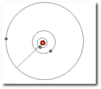
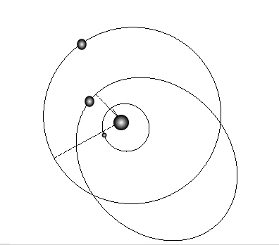
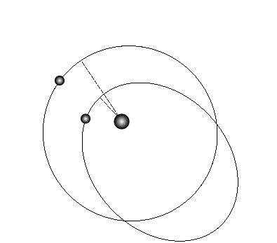
We’ve been looking into the possibility of detecting another planet in the system, and in order to do so, we’ve been studying synthetic data sets that contain the three known planets, as well as a fourth, potentially habitable planet in a potentially habitable orbit. The following table gives the parameters of our hoped-for system (which, like the real system, has its invariable plane inclined by 40 degrees with respect to the line of sight.)

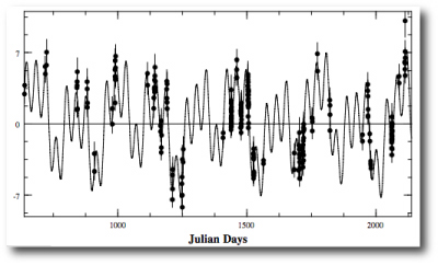
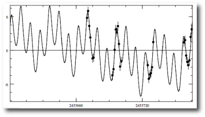
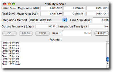
The first 155 points in the challenge data set used the actual observing times given in Rivera et al 2005. The remaining 32 points were generated using the version of Eugenio’s Keck_TAC program that we use to produce the systemic synthetic data sets. We then subtracted off the the first epoch time from all 187 observing times and multiplied each of the resulting times by the golden section, 1.618033989. This gives a system that has the dynamical characteritics of the real GJ 876 system, but with orbital periods that are all 1.618 times longer.

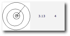
After setting up the uploads page on the backend, Eugenio uploaded the best fit that he was able to obtain, which had a chi-square of 3.13. A lot of computation went in to getting this fit, which took several days on a fast desktop machine.

Amazingly, the next day, user Roseundy submitted an even better fit,

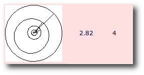
which brought the chi-square down to 2.82, with the following comment:

Arrrggghh!!!!!!!! I had this fit on Sep 13, but I thought the ChiSq was too high to bother to submit. Lesson learned.

Eugenio and I were quite excited. Systemic users have clearly gotten at least as good at fitting with the console as we are, and we have been thinking carefully about the problem for quite a while. In the comments section on Roseundy’s fit, Eugenio wrote:

Hi Roseundy, That is awesome work!! All the challenge systems will be based on some known model, possibly a random draw, some noise, and possibly other effects. The random draw and the noise complicate the situation for the modeler (me), so that knowledge of the model will not always result in the best fit. Actually, your result is a major success for the idea behind the systemic collaboration — distributing the process of fitting radial velocity data sets. Because I really don’t know precisely how the random draw and the noise affected the model, it may still be possible to get even lower chisq values. I encourage everyone to continue fitting this system (as well as others). It does require patience and perserverence.

Chris Thiessen wrote:

Roseundy, I’m very impressed. The two major planets have such different Keplerian and integrated fits that I was never able to get them to work well together. How did you get the two planet solution? I’m not sure I would have let the 48 day planet develop that much eccentricity if I’d seen a trend. Maybe I missed out that way. Great work!

Whereupon Roseundy revealed the secrets of his fitting method:

Once I saw how close the planets were, I realized I needed to work with integration turn on. This, of course, slowed things down painfully. To make progress, I cut down the dataset (the middle third of the velocity data) and played with that until I got a good (chi^2 of 7 or so) fit. I backed that out to the full data set (very painful) and then added additional planets based on the residuals. I polished until I got the fit you see. I’m sure it can be improved, but I lost patience with it. I would like to see three improvements to the console to make this easier in the future: 1. be able to subset the data 2. be able to select which planets are to be integrated together, using Keplerian calculations for the rest. this would help with systems where only a few planets substantially interact with each other 3. (my vote for the most important) a natively compiled console. java byte code may be portable, but I don’t it’s very optimized. Having optimized binaries (x86 on Linux preferably) would be a win, I think.

We agree. After the next release of the console, I think it would be a good idea to migrate to a strategy where the systemic community of users can work on the console code open-source style. This is clearly another area where a distributed attack will get important and interesting results.

In any event, thanks to everyone who has been reading the oklo blog and collaborating in the backend. We’ve had over 6,000 unique visitors so far this month, and the project is really starting to show promise.