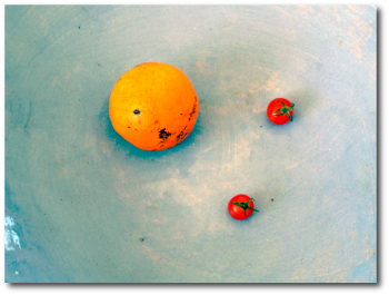
stability analysis

Rayleigh Taylor fingers

Image Source.

If you’re spending time on the collaborative systemic backend, you’ll know from the discussion threads that Eugenio has been making rapid progress on the downloadable console. He’s in the process of converting the code from a single-thread version to a fully multi-threaded package. Threading is important. It will allow the console to be gracefully reset in the event that a Levenberg-Marquardt polish takes more time than you bargained for, and it will allow for a variety of on-the-fly diagnostics regarding what’s going on under the hood.

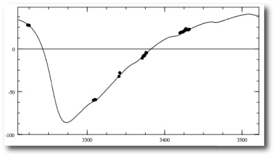
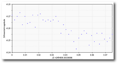
The latest version of the downloadable console now contains a multi-threaded orbital stability checker. To see it in action, download a fresh console (making sure to save your old systemic directory if you have built up a library of fits that you want to keep). I pulled up the HD 69830 dataset and quickly worked up a three-Neptune fit that is very similar to the fit reported by the Geneva team in their discovery paper.

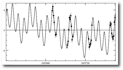
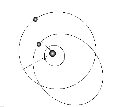
The two outer planets are roughly similar in mass to Neptune, while the inner planet, with a period of 8.66 days is somewhat less massive. It’s not immediately clear from looking at the orbital configuration:

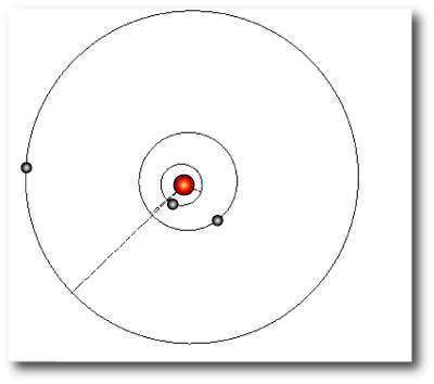
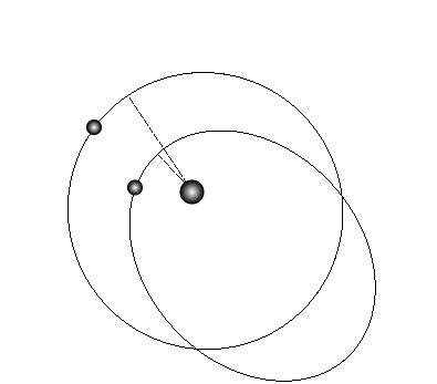
that this planetary troika is gonna get along to go along. A stability check is definitely in order. Clicking on the button for the long-term stability module:

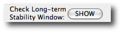
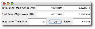
brings up a dialog window that you can use to control the stability integration. You specify the maximum timestep duration, the output frequency, and the integration duration and press go. At present, the console implements only a 4th/5th order Runge-Kutta integrator, but we’ll soon supply faster algorithms, including a Wisdom-Holman symplectic map:

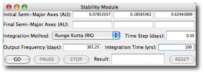
For this example, I specified a short 100-year integration (4200 inner planet orbits). This is enough to see whether the system is wildly unstable, but for a more diagnostic check, one would generally like to look at a longer duration (100,000 inner planet orbits, say).

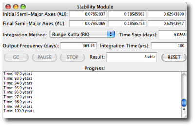
In this first implementation, a system is deemed “stable” if the semi-major axes of all the planets remain constant to within 1% of their initial values during the course of the integration. There are, of course, stable systems (such as a librating, equal-mass 1:1 resonance configuration) where larger semi-axis variations occur, but if semi-major axes vary by more than 1%, it means that considerable orbital energy is being traded back and forth, and the long-term prognosis is not good.

This HD 69830 3-planet fit easily lasts for 100 years. Nevertheless, as noted in the discovery paper, longer-term integrations show that the system is very close to the edge of stability.

I’m still working on the promised post about trojan planets. Look for it tomorrow!

And inside the second envelope…

Image Source.

First, a thank-you to everyone who submitted a fit to the second systemic challenge. I just loaded all the fits into the console and evaluated the chi-squares (with integration turned on). Jose Fernandes, of Lisbon, Portugal, submitted the winner, and will be receiving the $149.99 sky atlas from Sky and Telescope.

Jose’s fit has a reduced chi-square statistic of 3.94, and is comprised of three planets:

The outer two bodies have masses 1.58 and 0.5 times that of Jupiter, with eccentricities of 0.58 and 0.14. They share a common period of 362 days. The fit also has a tiny inner planet with a mass just under 3% that of Jupiter and a period of 50 days. This little guy improves the fit by wriggling the radial velocity curve up and down to statistically grab more points.

The system that actually generated the data was quite similar:

There are two equal-mass planets with masses 1.04 times that of Jupiter, with eccentricities of 0.7 and 0.2. They share a common period of 365 days. The 50-day planet in the winning fit was spurious, as is often the case when a model planet has a mass that is far smaller than its companions.

This system is an example of a one-to-one eccentric resonance. It is based on a system that was discovered by UCSC physics student Albert Briseno in one of the simulations that he ran for his undergraduate thesis, and it was formed as the result of an instability in a system that originally contained more planets. The system experienced a severe dynamical interaction, which led to a series of ejections. After the last ejection, two planets remained. They share a common orbital period, and gradually trade their eccentricity back and forth. Their interaction gives a strong non-Keplerian component to the resulting radial velocity curve for the star, which makes this a tricky system to fit. While the system might seem absurdly exotic, it’s recently been suggested by Gozdziewski and Konacki that HD 82943 and HD 128311 might have their planets in this configuration (you can of course try investigating this hypothesis for yourself with the console). Their paper is here.

The challenge 002 system is an example of a general class of co-orbital configurations in which the two bodies constitute a retrograde double planet. If you stand on the surface of either world, the other planet appears to be making a slow retrograde orbit around your moving vantage as the libration cycle unfolds over several hundred orbits.

In tomorrow’s post, we’ll stay on the topic of co-orbital planets, and look at some interesting new work by Eric Ford on the possibility that we might soon be able to observe planets in Trojan configurations. Two planets in a Trojan orbit librate around the points of an equilateral triangle in the rotating frame. Indeed, when such an arrangement occurs, it’s possible that a particularly interesting dataset might have the capacity to launch a thousand fits.

[For more about 1:1 resonances, see this post and this post. For a discussion about the audio wave forms that they produce, see this post.]

CfA

Image Source.

Back from a great visit to the Harvard CfA. The exoplanet research effort out there is amazingly comprehensive, and I soaked up a whole range of interesting news items to report. A slew of posts are in the works.

I’ve uploaded my colloquium talk in (1) Apple Keynote format (harvard.key.tar.gz) , (2) Powerpoint format (harvard.ppt.tar.gz), and (3) as a set of .pdfs. The talk was built in Keynote, and thus will look best in that format. Note that the Keynote and Powerpoint files are both quite large (~58MB compressed, ~90MB uncompressed) because they contain a variety of animations. The .pdfs amount to about 7 MB, and show only the splash frames from the animations. Feel free to use any of these slides in presentations or classes (with a shout-out to oklo.org).


Eugenio has been working hard on the console during the past few days. The downloadable version now contains a stability checker which integrates a fit for a user-specified period. Relative changes in the semi-major axes of more than 1% are then used to flag instability. Give it a whirl! We’ll discuss it in more detail in an upcoming post.

Tomorrow, I’ll announce the results of the second systemic challenge. The third challenge system is already available on the downloadable console.

Some updates

Image Source.

I’ll be gone on a trip to the Harvard CfA for the next several days. While I’m there, I’ll be giving a colloquium talk, and in addition, I’ll be trying to extract all the latest research news items from the CfA’s large group of exoplanet researchers. That’ll likely give me some stuff to write about in upcoming posts.

We’ve now closed the Systemic Challenge 002 contest, and I’ll tally up the results on the plane ride home. Look for a post this weekend that will explain what’s going on in the Challenge 002 data set. Eugenio has cooked up a great batch of RVs for the Challenge 003 system, and we’ll be releasing them this coming weekend.

Note that the dates of the challenges are slipping from what was announced in the S&T article. There’ll still be a total of four systems, but the contests will run over two months rather than one as originally planned. As soon as the contests are finished up, we’ll release the “Systemic Jr.” set of 100 trial systems. Based on our experience with these systems, we’ll make any necessary modifications to the simulation profile, and then we’ll be set to start the long-promised full Systemic simulation. In the meantime, keep submitting fits! I’d really like to see the chi-square come down on a dynamically stable configuration for 55 Cancri.

In other news, we’ve now got confirmations for both WASP-1b and WASP-2b.

On Monday, Mike Fleenor, of Volunteer Observatory in Knoxville Tennessee wrote:

I observed a complete transit of WASP-1b last night under very good conditions. My LC shows mid-transit very close to your predicted center. Details are available here.

Last weekend, Joe Garlitz from Elgin Oregon wrote:

Last night (Fri/Sat) I tried for WASP2 and got some data that looks promising. The data is very noisy and I would not feel comfortable about presenting it without some other confirming (hopefully someone else got data) observations.

I have attached a .jpg image of the data chart. The data is really forced to get any kind of “curve”. The solid line represents a running average over 16.25 minutes, 13 data points.

The individual images are 65sec at an interval of 75 sec. The scope is 200mm @ f/8 with a Cookbook 245 CCD, no filters.

Here’s his lightcurve:

Today, Geir Klingenberg from Norway checked in with a confirmation of Garlitz’s result (which he obtained remotely from a telescope in New Mexico:

Hi Joe,

I observed the ingress of this WASP-2 transit, see here.

Seems to fit your data nicely.

I used a robotic telescope at GRAS: 0.3m SCT @ f/11.9 and a FLI IMG1024.

Way to go, guys!