HD 208487

Image Source.

An relevant paper showed up on the astro-ph preprint server this morning, “A Bayesian Kepler Periodogram Detects a Second Planet in HD 208487” by P. Ç. Gregory of the University of British Columbia.

Gregory employs a technique known as the parallel tempering Markov Chain Monte Carlo algorithm to argue that the HD 208487 data set contains two planets. The first planet (which was previously announced by Tinney et al. 2005, and confirmed by Butler et al. 2006) has a period of 130 days and a minimum mass 37% that of Jupiter. The second planet in Gregory’s model lies out at a period of 908 days, and has 46% of Jupiter’s mass.

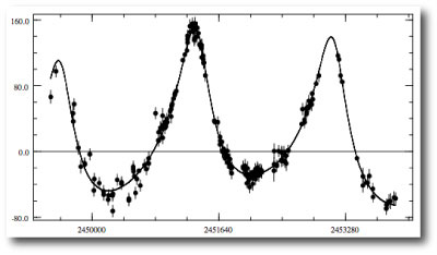
Interestingly, the console does not recover Gregory’s parameters precisely, but it does find a fit that’s extremely similar. (I just uploaded the fit to the systemic back-end.) The radial velocity reflex curve looks like this:


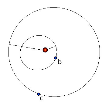
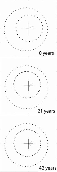
wheras the planetary configuration (at the moment when the first radial velocity data point was obtained on Aug. 8th, 1998) looks like this:

It’s interesting to look at the fits for the latest HD 208487 dataset that have been submitted by participants in the systemic collaboration. At the moment, there are six different fits:

On September 4th, mikevald submitted a 2-planet fit that is a close analog of the one published by Gregory. In the last several days, dstew and andy have also turned in fits that have essentially the same configuration as obtained by Gregory. That’s definitely cool.

In addition to the five fits that look like the Gregory configuration, with the outer planet at a period of P~1000 days, there’s also a completely different take on the system that was submitted this morning by Olweg. In the Olweg fit, the second planet lies interior to the known planet, and has a period of only 29 days. The chi-square is less than one, indicating a slight degree of overfitting. When overfitting occurs, it can easily be remedied by a slight random perturbation of the parameters. It’s very interesting that this fit was completely missed by the Bayesian Kepler Periodogram, so I thought I would have a closer look at Olweg’s model system.

The Olweg radial velocity curve is radically different from the Gregory fit:

The 28.68 day inner planet has a mass of 0.16 Jupiter masses (about 50 Earth masses) and travels on an orbit of modest (e=0.18) eccentricity. There’s a fair amount of planet-planet interaction in this system over the time scale of the radial velocity observations. By the time the fit reaches the end of the data set, there’s a noticeable difference between the keplerian model fit and a self consistent (integrated) model fit:

The system is stable, however, when I did a short test integration of 100,000 years. The secular interaction between the two planets causes the two orbits to execute a complicated dance over a timescale of several thousand years, with the periastron angle of the inner planet orbit mostly librating around an anti-aligned configuration.

As I’ve remarked in an earlier post, we’re currently in the progress of upgrading the downloadable console so that it will be capable of computing estimates of the uncertainties in the orbital elements of a fit. A good way to generate uncertainties in this context is to use the so-called bootstrap method. In the bootstrap, one re-draws the original radial velocity data set with replacement, thus producing alternate realizations of the data in which a fraction of the points appear more than once, and in which a fraction do not appear at all. One then fits to these new datasets, thereby building up distributions for each orbital element. (For more detail, see this paper, which describes in detail how this procedure was applied to the radial velocity data set for HD 209458.) When I run a self-consistent bootstrap analysis based on the Olweg fit, I get the following mean values and standard deviations for the parameters:

This fit is thus quite well constrained, and is a completely viable competing model for describing the hd208487 planetary system. I think the situation here really underscores the value of the systemic collaboration. Many radial velocity data-sets can be fitted by completely different models that offer equally robust fits to the data, while simultaneously maintaining small uncertainties on their bootstrap-estimated parameters.

So how do we know which HD 208487 system (if either) is correct? I’m hoping that the Monte Carlo simulation that will make up phase II of the systemic project will give a great deal of insight into when a particular orbital model can be deemed secure.

desiderata

strands of wheat

Image Source.

It’s good to see that users are still streaming into the systemic collaboration, and activity on the back-end is staying strong. The catalog of submitted radial velocity fits is now approaching 1,000 entries, and nearly every data-set has at least one fit. We need more users, though. Both Stefano and Eugenio have been working very hard behind the scenes to engineer improved usability for the site. There are a lot of items that are still on our plate, but progress is definitely being made.

We can now internally query the database of submitted fits to statistically characterize the planetary models that are being submitted. Once this functionality is fully tested, it’ll be made available to all users on the site. For example, here’s a plot of eccentricity vs. period for all of the fits submitted with 0.8 < chi-square < 2.0: aggregated P-e diagram

It’s interesting to compare this with the plot that one can produce at exoplanet.eu based on the static catalog of published planets:

One immediately notices that the diagram produced from the back-end data is populated in the upper left hand corner, whereas this region in the published catalog is completely cleared out. Note that planets in this region are known from theoretical arguments to be tidally circularized… (tune in soon for more on that issue).

One final note. The downloadable console is now much lighter. The large filesize of the previous version was due to the very extensive synthetic data sets for alpha Centauri. If you want the alpha Centauri velocities, the fully loaded console that contains the alpha Centauri data is here. Within a day or so, we’ll be updating the downloads page to reflect this change and to give more guidance for International Windows users.

TrES-2 follow-up

The transit game is getting to be a competitive global business. No sooner is a new transit announced than amateur astronomers worldwide are on the sky to obtain follow-up observations. Tonny Vanmunster, of Landen Belgium and Ron Bissinger of Pleasanton California are generally among the first to check in with confirmations. Vanmunster nailed TrES-1 a mere week after its announcement in 2004. Last summer, Bissinger caught HD 149026b on literally the day it was announced. In the case of TrES-2, which was announced yesterday, it looks like Vanmunster has snagged the prize. “What’s up, Cali?”

[Actually, it was both cloudy and the middle of the day in Pleasanton while Vanmunster was on the sky. But there’s a transit tomorrow night, Sept. 10/11 PDT, that Ron’ll likely catch.]

Here’s Vanmunster’s light curve. The transit was in progress at dusk in Belgium, so he was able to observe only the latter part of the event.

Vanmunster writes:

Here are some technical details : observations were made at CBA Belgium Observatory, using two 0.35-m f/6.3 Celestron telescopes, each equipped with an SBIG ST-7XME CCD camera. I simultaneously made unfiltered and R-band observations (hence the 2 telescopes). The included light curve is unfiltered, and each dot in the curve is the average value of 5 successive observations (binned). The gray lines show the standard deviation (about 4 millimag on average). Exposure time was 15 to 20 sec.

The egress is very evident in the light curve, and happened right at the predicted time. The transit depth was approx. 0.0155 mag, which again corresponds well with the value published in the discovery paper.

Follow-up observations such as the ones made by Vanmunster and Bissinger can be very scientifically useful. For example, Vanmunster’s 2004 observations allowed us to get an improved estimate of the TrES-1 planetary radius, and he co-authored a journal article with us on that topic. Both Vanmunster and Bissinger were involved in the discovery of X0-1, and both are co-authors on the recent Shankland et al. paper which I’ll talk up in an upcoming post.

TrES-2

TrES-2

Image Source.

When I teach Astronomy 101, I like to brag about my weight early and often during the class. For example, when I introduce the concept of energy, I’ll tell the students, “Let’s say you have a guy like me. You know, six foot three, 285 lbs (129 kg)… pause… If I’m running down the street at 9 meters per second, then my kinetic energy is 10,449 Joules.”

The first time that I floss my weight, there’s usually a slight rustle through the lecture hall, but generally nobody says anything. Students in the back row glance up slightly startled from their online poker games, then adjust their hoodies and ante up for the next hand.

As the quarter progresses, I’ll find other opportunities to claim an outrageous heft. “Take me, for example, I weigh 287 lbs… pause… solid muscle.”

Usually, that line finally gets a rise out of someone, “You don’t weigh 287!” they’ll blurt out, “You’re more like 150!”

“Are you challenging me?” I’ll roar, “Anyone want an F on the next exam?” Nervous laughter. Eventually, a few more classes in, everyone just rolls their eyes when I remind them of my outrageously high mass.

Eventually, when I get all the way out to the galactic scale, I reach the topic of dark matter and I can cash in on the long set-up. “Look at that rotation curve!” I’ll say, “The orbital velocities of the galaxies in this cluster suggest that there’s many times more mass present than we can observe in the form of stars. It’s like [pause] It’s as if some guy who looks like he weighs 160 steps on the scale and it turns out that he actually weighs 285.”

They laugh and the joke works because we’re able to look at a person and make a mental estimate of their mass. When it comes to extrasolar planets, however, judging mass by size has proved to be effectively impossible. If you are in the vicinity of a hot Jupiter, and are able to measure its radius, you’ll have little basis for judging how massive it is. That is, the mass-radius relation for hot Jupiters isn’t a single-valued function, and we don’t know why. Indeed, understanding the radii of the known transiting planets is one of the most currently interesting exoplanet research topics.

I’ve written several oklo posts about the size problem for the short-period extrasolar planets [see here, here, here, here and here]. In a nutshell, within the aggregate of transiting exoplanets that orbit stars bright enough for high-precision follow-up, there’s a full range of size discrepancies. HD 149026 b is much smaller than would be predicted for a standard-issue Jovian planet of its mass and temperature. TrES-1 has a radius that agrees very well with the theoretical predictions. HD 189733 is somewhat on the large side, and HD 209458 b, famously, is much larger than predicted. [In tomorrow’s post, I’ll give an update on the hydrodynamical simulations that we’ve been doing with the goal of eventually sorting out whether HD 209458 b is caught in Cassini state two.]

It’s therefore still a big deal whenever a new transit is discovered in association with a bright parent star. Today, the TrES collaboration, (who bagged TrES-1 back in ’04) are rolling out a new transiting planet — TrES-2.

TrES-2 is a more-or-less standard-issue hot Jupiter. At 1.28 Jupiter masses, it’s a little more massive than the average short-period planet, and its orbital period of 2.47 days is slightly shorter than the 3-day average period exhibited by this class of objects. The TrES-2 parent star is very similar in mass, radius, and temperature to the Sun. It lies in Lyra, and has a V-band magnitude of 11.4 (making it ideal for follow-up observations by amateurs — check out the transitsearch.org ephemeris table here).

Turns out that TrES-2 is on the large side. Our theoretical models predict a radius of 1.07 Jovian radii if the planet has a core, and 1.11 Jovian radii if it is core-free. The measured radius is 1.24 Jovian radii, with a lower error bar of 0.06 Jovian radii. The planet is thus a bit more than 2-sigma larger than the core-free model, and provides evidence that the mechanism responsible for providing extra heat (and expansion) to these planets is a relatively generic and commonplace phenomenon. It’s hard to invoke special purpose explanations for HD 209458 b’s radius when there’s a slew of other transiting planets that suffer a similar bloat.

One reason I like transiting planets is that they can be drawn to scale with their orbits and parent stars. In TrES-2’s case, the geometry looks like this:

TrES-2 system to scale

With Illustrator’s scale tool, it’s easy to insert TrES-2 into our planetary police line-up:

Five for the show

Curiously, the TrES-2 paper makes no mention of the metallicity of the TrES-2 parent star. The metallicity is of great interest because it will allow a test of the Guillot et al. hypothesis that the planetary radii are the result of a concentration mechanism that greatly amplifies the overall solids content of short-period exoplanets that orbit high-metallicity stars. I asked Dave Charbonneau if his team had anything up their sleeve in the metallicity department. He told me that they haven’t had time to get an accurate measurement, and that the number will be released in a follow-up paper.

Amazingly, TrES-2 lies in the field of view of the Kepler Mission. This means that the Kepler satellite will make repeated high-precision measurements of the TrES-2 light curve, with a photometric precision of about one part in 10,000 and a cadence of 15 minutes. This data will allow for very accurate determinations of the durations between transits. By observing small variations in the orbital period, you can detect other bodies in the system, in many cases with masses down into the terrestrial regime. The process by which this is done is highly analagous to the multiparameter fitting process that one uses when running the console, with transit intervals playing an analogous role to the usual radial velocity measurements. Once we get our plate cleared of current console improvements — integrator, bootstrapper, multi-threading, etc. etc., we’ll reconfigure it to enable a look at planet detection via transit timing.

New Texas V’s

Image Source.

Data data data. Robert Wittenmyer and his colleagues at the University of Texas have just posted a paper on astro-ph that contains a slew of new radial velocities for several famous planet-bearing stars, including 47 UMa, 14 Her, and 16 Cyg B. The velocities are all tabulated in the paper, so we’ll have them up on the systemic backend very shortly. [I’ll post a comment to this post when they’re up on the site. If you’re totally gung ho to get them right away, you can extract them from the posted latex file at astro-ph, and then add them manually to systemic’s datafiles directory.]

We always try to add new radial velocity data sets as soon as they become publicly available, and lately, these updates have been occurring roughly once per week. For the time being, the simplest way to get your fresh V’s is to rename your old systemic directory, and then download a new console. When the new console and catalog data are downloaded and unzipped, you can copy any previous fits and soundfiles that you’ve created into the new fits and soundClips directories.

The data in the Wittenmyer paper come from both the Harlan J. Smith 2.7-meter telescope and the Hobbey-Eberly 9.2-meter telescope. The cadence of the Smith telescope observations typifies the usual pattern of radial velocity survey data. The individual points are spaced essentially randomly in time, with many days separating each point. The Hobbey-Ebery data, on the other hand, are quite different. These data are much more densely sampled, and many nights contain several velocities in succession. In many stretches, the star is observed every few nights. This pattern results from queue-scheduling, which enables very intensive monitoring of systems that are of particular interest. I think queue scheduling is the wave of the future, and in the systemic simulation, we’ll have many synthetic data sets whose cadences correspond to the queue-scheduled approach.

The most prominent planet orbiting 14 Her has been known since the late 1990s. This world, known as 14 Her “b”, has a minimum mass about 4.6 times that of Jupiter, and a period of ~1770 days. If it were in our solar system, it would orbit in the asteroid belt. The parent star 14 Her is about 90% as massive as the Sun, and is more than twice as metal-rich. Given the planet-metallicity connection, it’s absolutely no surprise that 14 Her has a heavy-duty planetary system. I bet that 14 Her “b” has a very interesting system of satellites.

It’s pretty clear from the one planet fit that 14 Her “b” is not the only planet in the system, and over the weekend, several systemic users have submitted interesting fits to the data that reduce the chi-square by adding a second planet. For example, on August 30, user mikevald uploaded a two-planet fit in which the second planet, 14 Her “c”, has a period of 6159 days and an eccentricity e=0.52. This model currently fields the lowest chi-square statistic of any of the submitted 14 Her fits. The orbits in this best-fit system are crossing, however, indicating that the model may not be dynamically stable over the long run. On September 5th, allanfloering submitted a fit with nearly as good a chi-square, in which the outer planet has a 14,669 day period and an eccentricity e=0.09. Allanfloering’s world, if it exists, lies 11.77 AU from 14 Her, out at a Saturn-like distance.

Wittenmyer et al. show that the addition of their new 14 Her data suggests that 14 Her “c” has a period of order 6900 days, albeit with a low eccentricity. In their models, “c” and “b” may be participating in 4:1 resonance. A quick fit on the console with the Wittenmyer et al data included gives a radial velocity curve that looks like this:

corresponding to a planetary configuration that has an outer planet with a modest eccentricity e=0.20.

As soon as the data go up on the site, feel free to try working up improvements. It will be interesting to see how many fits to the full 3-telescope data set are participating in 4:1 resonance.

Web 2.0

fenceposts at ucsc

Hey ya’ll, there’s a whole lotta fittin’ goin on out there in the back 40.

Seriously, though. We’re really seeing a great response from users who are contributing their efforts. Nearly 200 people have registered on the back-end during the past few days, and over 750 different radial velocity fits have been uploaded. Hopefully we’ll see that work continue to flow in, and everyone has been showing admirable patience as we smooth out the inevitable rough spots which began to show up as soon as we had a surge of real users on the site.

If you’re arriving by way of the Sky and Telescope article, you’ll notice that the full universe of 100,000 synthetic stars is not yet listed on the systemic backend. During September, we’re still carrying out the first phase of our planned research effort, which consists of accumulating a wide variety of fits to the full collection of actual, published radial velocity data sets. Very soon, we will have accumulated enough fits to be able to present a dynamic, interactive catalog of candidate planets. A query-based dynamically generated planetary catalog will allow a variety of very interesting questions to be answered. For instance, by how much can one deflate the famous eccentricity-period diagram, while still demanding a prespecified goodness-of-fit for all of the candidate planets?

generated at exoplanet.eu

At the moment, such questions are hard to answer, because (other than here at oklo) there is no consolidated repository of radial velocity data and associated self-consistent fits.

In order to make dynamically generated planet catalogs scientifically useful, we’re going to have to provide several more tools to the users. As I mentioned yesterday, the console will soon be multi-threaded, which will make it easier to use for high-performance work. In the interim, however, you can have the console print a stream of diagnostic messages by launching it from the command line. For example, on linux or OSX architectures, open a terminal (shell), cd to the systemic directory, and type java -jar systemic.jar at the prompt . The diagnostics provide a running update of the progress of the console as it produces fits to the data set.

We’ll also soon be providing a long-term integration window that will allow users to verify that their model systems are dynamically stable. It’s alarmingly easy to find multiple-planet fits to radial velocity data sets that have low values for the reduced chi-square statistic, but in which the planets experience dynamical disasters (collisions, ejections, close encounters, etc.) on a time scale that is short in comparison to the known age of the parent star. Indeed, most of the candidate stars in the back-end catalog are more than 2 billion years old. Young stars tend to be rapidly rotating, which broadens their absorption lines and makes radial velocity measurements less accurate. Rapidly rotating stars also tend to have elevated levels of magnetically driven chromospheric activity, which adds additional noise to the velocity estimates.

And finally, the console needs to provide error estimates on the orbital parameters that it generates. This is best done using the so-called bootstrap method, which we’ll discuss in an upcoming post.

Systemic Challenge — data set #1

Image Source.

We’re continuing to see a strong influx of new users and activity on the systemic backend. Thanks to everyone who’s taking part! If you’re a first-time visitor to the Systemic Project website, please read the weblog entries that follow this post. They contain the information you need to start participating, and they give a recent day-by-day overview of the project developments.

Now that we’ve got an active user-base for the systemic console, we’re pleased to release the first Systemic Challenge synthetic radial velocity data set. This data set corresponds to a realistic simulated planetary system that is both scientifically interesting and non-trivial to fit.

Sky and Telescope is sponsoring the world’s first radial velocity fitting contest in connection with our challenge system. The person who submits the self-consistent (integrated) fit to the data having a chi-square value closest to one will receive a paperback edition of the Millennium Star Atlas (a $149.95 value).

Continue reading

consolidation

Image Source.

Wow! The American Scientist and Sky and Telescope articles are clearly getting the word out. We’ve been seeing a significant increase in traffic on the oklo.org site, both in terms of visits (yellow bars) and bandwidth and page views (green and blue bars). The bandwidth increase is especially gratifying. It reflects the fact that many users are registering on the back-end, downloading the console, and submitting fits. As I write this, new and interesting fits for a variety of different radial velocity data sets are rolling in to the star catalog. Our goal of fostering original, public-participation exoplanet research is starting to be realized, and I want to thank everyone who’s lending a hand.

Late August stats.

If you’re a first-time visitor to the Systemic Project website, please read the blog entries that were posted prior to this entry. They contain the information you need to start participating, and they give an overview of the current project status. If you are a return visitor, please have a look at the updated back-end. Stefano has made a number of code and design improvements that streamline the workflow and make the site easier to navigate.

On to some planet issues. The Mu Ara (HD 169061) system, which contains four known planets, is shaping up to have significant implications for the systemic project. Intense interest in the system has been spurred by a recent paper from the Swiss group (Pepe et al. 2006) that presents a self-consistent 4-planet model. Pepe et al.’s orbital fit (given in their Table 1) provides an excellent match to the radial velocity data sets, but when they carried out a long-term integration of the system, they found that the gravitational interactions between the planets lead to catastrophe after 76 million years. The parent star Mu Arae has an estimated age of 6.4 billion years, so clearly we don’t yet have a full understanding of what’s going on with this system.

The discord within the Pepe et al. model is provided by the two middle planets, one of which has a 310 day orbit, and the other which orbits in 643 days. The planets are on the edge of the 2:1 mean motion resonance, with the practical consequence that they experience a strongly chaotic orbital evolution. The orbits change eccentricity and orientation on a timescale of only decades:

I’ve made a movie that tracks the evolution of the orbits over 528 years. Here are links to a .mov version (288 kB) and an .mp4 version (1.5 MB). It’s clear from the movie that the interaction is both complicated and unpredictable. The planets display no catastrophic excursions on the 500 year timescale of the movie, but eventually, they experience orbit crossings leading to a likely ejection of the inner 0.5 Jupiter mass planet.

The Mu Ara dataset HD169061_B06P06CH on the console back-end combines both the Pepe et al. data as well as the most recent data from Butler et al. 2006. I’m hoping that someone can get a stable, self-consistent, low chi-square fit to this combined data set. Such a fit would give the best available view of what’s going on with the system, and would underscore the scientific relevance of the systemic project.