When it comes to planetary systems, our own eclectic gathering of eight (or nine, or ten) planets is by far and away the best characterized and best understood. We’ve flung space probes past all of the planets in the solar system, and we’ve directly, physically, probed four of them (in addition to two major satellites). We know their orbits to stunning, uncanny precision. We have actual pieces of Vesta and Mars under minute scrutiny in our laboratories. We have coffee table books overflowing with detailed photographs our our home worlds.

I can step right outside my door and photograph the surface details of a habitable terrestrial planet.

Sadly, we don’t have anything rembling this wealth of detail when it comes to extrasolar planets. Most of our information is encapsulated in the tables of radial velocity measurements accessible to the Systemic Console. Much of what I write about in these posts, and indeed, most of what we can infer about these distant worlds, must be squeezed from sparse columns of times, velocities, and velocity uncertainty estimates.

Without question, the most valuable radial velocity data belongs to the red dwarf GJ 876. Lying a mere 15 light years away in the direction of the constellation Aquarius, GJ 876 is accompanied by three known planets. Two outer Jovian planets orbit in a 2:1 mean-motion resonance with periods of 30 and 60 days. Further in, much closer to the parent star, is a strange world with 7.5 earth masses, circling on an orbit that lasts only 1.93776 days.

Systemic team member Eugenio Rivera was the lead author on the paper that announced the discovery of the bizzare inner planet orbiting GJ 876. The discovery was big news last summer, involving a press conference at NSF Headquarters in Washington DC, and landing Dr. Rivera squarely in the June 15th, 2005 issue of the New York Times.

Although the media glare focused almost entirely on the dramatic extraction of the inner planet from the radial velocities (to replicate this feat, try systemic console tutorial #3), Eugenio’s paper contains a number of other very significant, albeit subtler results. Perhaps the most important of these is the fact that the orbital inclination of the GJ 876 outer-planet orbits can be determined to a very high accuracy from the analysis of the radial velocity data. There are no other radial velocity data sets for which this is possible, and it seems unlikely that this situation will change for at least a decade.

In general, when a planet is on a Keplerian (that is a purely elliptical) orbit, the radial velocity method allows one to measure the mass of the planet multiplied by the sine of the inclination angle of the planetary orbit. [The convention in dynamical astronomy is for the inclination angle, i, to be reported with respect to the plane of the sky. Hence, an inclination i=0 deg corresponds to an orbit that is being viewed face-on, wheras an inclination i=90 deg corresponds to an orbit that’s being viewed edge on. This convention for inclination differs from the convention that we use when we talk about planetary orbits in the solar system. In the solar system, an orbital inclination I=0 refers to an orbit that lies in the plane of the solar system. I find this a more intuitive way to think, and so at oklo.org, when I refer to an orbital inclination, (capitalized) I, of zero degrees, I have in mind a system whose orbital plane is aligned with our line of sight to the star.]

Because the Doppler velocity method tracks only a component of the star’s velocity, it cannot distinguish between a massive planet whose orbit is being viewed nearly face-on (I=90) and a lower-mass planet whose orbit is being viewed close to edge-on (I=0). In the GJ 876 system, however, the interactions between the two planets are so strong that the radial velocity fit changes perceptibly as the (assumed) co-planar inclination of the system varies. One can therefore estimate the inclination by systematically testing values for I, and seeing whether the fit improves or gets worse. By doing this, and by making a careful analysis of the errors, Eugenio was able to show that if the outer two planets are orbiting in nearly the same plane (which we believe to be an extremely reasonable assumption) then the tilt of that plane with respect to the line of sight to the star is 40 degrees plus or minus 3 degrees.

Shown just below is a figure that charts how our ability to measure the co-planar orbital inclination for GJ 876 b and c has improved over the observing seasons from 1999 to 2004. As more velocities are accumulated, the location of the minimum value of the chi-square statistic of the fits gradually becomes increasingly better-defined. By the end of 2004, the position of the minimum could be located to within three degrees (1-sigma). As more data comes in, it will become possible to additionally observe whether the outer two planets have a small mutual inclination. Theories of migration (for example this paper) predict that the mutual inclination between the two outer planet orbits should be very small, likely only a few degrees.

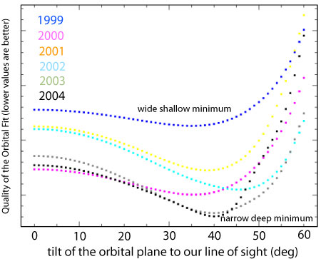
The plot above was reworked for the oklo format from this original postscript version that Eugenio produced yesterday. Although the figure above doesn’t show it, the latest 2005-2006 data provides an impressive further improvement. Eugenio will be writing a short paper the latest results for the Astrophysical Journal, and when it passes peer review, oklo.org readers will be the among the first to see the results. Also, in the comment thread to this post, I’m put a technically detailed discussion from Eugenio about the assumptions that went into making the above figure, and some of the conclusions that can be drawn from it.